Let's reproduce GPT-2 (124M)
Description
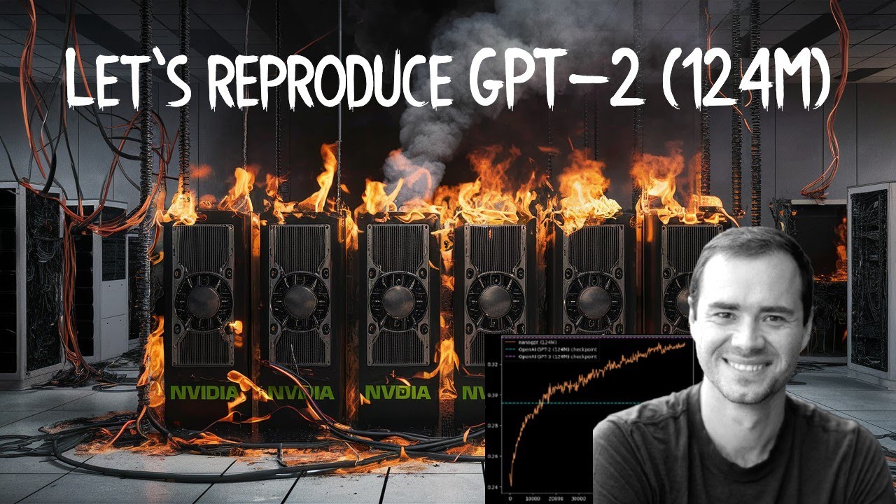
We reproduce the GPT-2 (124M) from scratch. This video covers the whole process: First we build the GPT-2 network, then we optimize its training to be really fast, then we set up the training run following the GPT-2 and GPT-3 paper and their hyperparameters, then we hit run, and come back the next morning to see our results, and enjoy some amusing model generations. Keep in mind that in some places this video builds on the knowledge from earlier videos in the Zero to Hero Playlist (see my channel). You could also see this video as building my nanoGPT repo, which by the end is about 90% similar. Links: - build-nanogpt GitHub repo, with all the changes in this video as individual commits: https://github.com/karpathy/build-nanogpt - nanoGPT repo: https://github.com/karpathy/nanoGPT - llm.c repo: https://github.com/karpathy/llm.c - my website: https://karpathy.ai - my twitter: https://twitter.com/karpathy - our Discord channel: https://discord.gg/3zy8kqD9Cp Supplementary links: - Attention is All You Need paper: https://arxiv.org/abs/1706.03762 - OpenAI GPT-3 paper: https://arxiv.org/abs/2005.14165 - OpenAI GPT-2 paper: https://d4mucfpksywv.cloudfront.net/better-language-models/language_models_are_unsupervised_multitask_learners.pdf- The GPU I'm training the model on is from Lambda GPU Cloud, I think the best and easiest way to spin up an on-demand GPU instance in the cloud that you can ssh to: https://lambdalabs.com Chapters: 00:00:00 intro: Let’s reproduce GPT-2 (124M) 00:03:39 exploring the GPT-2 (124M) OpenAI checkpoint 00:13:47 SECTION 1: implementing the GPT-2 nn.Module 00:28:08 loading the huggingface/GPT-2 parameters 00:31:00 implementing the forward pass to get logits 00:33:31 sampling init, prefix tokens, tokenization 00:37:02 sampling loop 00:41:47 sample, auto-detect the device 00:45:50 let’s train: data batches (B,T) → logits (B,T,C) 00:52:53 cross entropy loss 00:56:42 optimization loop: overfit a single batch 01:02:00 data loader lite 01:06:14 paramet
Summary
Generated by gpt-5.6-solAt-a-Glance
- Verdict: Watch fully
- Core thesis: A faithful GPT-2 124M can be rebuilt from first principles in compact PyTorch, accelerated roughly 11x on one A100, scaled to eight GPUs, and trained on modern data to surpass OpenAI's checkpoint on the demonstrated validation and HellaSwag comparisons.
- Why it matters: The video is an unusually complete systems-level walkthrough of transformer implementation, training correctness, GPU optimization, distributed execution, data preparation, and evaluation—including the subtle failure modes that determine whether a model-training run is valid or merely fast.
- Best use: Use it as an implementation and review checklist while building or auditing a compact pretraining stack; follow the accompanying code and commit history rather than treating it as a purely conceptual lecture.
Executive Summary
Karpathy reconstructs GPT-2 124M in fewer than 100 lines of core model code, first proving architectural compatibility by importing Hugging Face's converted OpenAI weights and reproducing coherent generation. The model uses a 1,024-token context, 50,257-token GPT-2 vocabulary, 12 transformer blocks, 12 attention heads, and 768-dimensional embeddings. He explains GPT-2's decoder-only, pre-normalized residual architecture as alternating communication through attention and per-token computation through the MLP.
He then converts the implementation into a correct training system: shifted next-token targets, cross-entropy loss, AdamW, weight tying, GPT-2-style initialization, residual-path scaling, gradient clipping, cosine learning-rate decay with warmup, selective weight decay, and gradient accumulation. Several details are presented as correctness traps, including device movement semantics, zeroing accumulated gradients, dividing micro-batch losses during gradient accumulation, and synchronizing distributed gradients only on the final accumulation step.
The systems optimization section shows that advertised arithmetic throughput is not the same as realized training speed because transformer workloads are often constrained by memory movement. On one A100, TF32 cuts the demonstrated step time from roughly 1,000 ms to about 300 ms; torch.autocast with bfloat16 adds a smaller gain; torch.compile reduces it to about 129 ms; FlashAttention reaches roughly 96 ms; vocabulary padding and fused AdamW bring it to about 90–93 ms. The cumulative improvement is approximately 11x before scaling to eight A100s with DistributedDataParallel, where the run processes about 1.5 million tokens per second.
For substantive pretraining, he replaces Tiny Shakespeare with the 10-billion-token FineWeb-Edu sample, tokenizes it into 100 shards of 100 million tokens, and adds validation, sampling, logging, and HellaSwag evaluation. A one-epoch, 10-billion-token run surpasses the released GPT-2 124M checkpoint on his FineWeb-Edu validation loss and HellaSwag setup; a 40-billion-token overnight run nearly reaches the cited GPT-3 124M HellaSwag result. He explicitly warns that these are not clean apples-to-apples claims: the data distributions differ, benchmark contamination is possible, and an unshuffled data loader creates suspicious periodic loss behavior.
Key Takeaways
- Claim: Architectural fidelity should be verified by loading a known checkpoint before attempting training from scratch. | Evidence: The custom GPT-2 implementation mirrors Hugging Face's parameter naming, imports the converted OpenAI tensors—including manually transposing TensorFlow-oriented weights where required—and produces the same outputs as direct use of the Hugging Face model code, even though the higher-level Hugging Face pipeline's generation defaults were not exactly reproduced. | Implication: For any internally implemented model or agent component, establish a reference-equivalence test against a trusted implementation before optimizing, distributing, or retraining it. | Caveat: Matching coherent samples alone is insufficient because sampling settings such as top-k and other hidden pipeline defaults can change generations; direct logit or model-output comparison is the stronger check.
- Claim: Training correctness depends on small implementation details that can silently alter the effective objective. | Evidence: The walkthrough catches a CPU/GPU tensor mismatch, emphasizes that tensor.to(device) returns a new tensor, requires optimizer.zero_grad because backward adds into gradients, and demonstrates that gradient accumulation only matches a large batch if each micro-batch loss is divided by the number of accumulation steps. | Implication: Ken should require toy-case equivalence tests for accumulated versus full-batch gradients, single- versus multi-GPU results, device placement, and optimizer state before trusting larger training or fine-tuning jobs.
- Claim: Memory traffic and kernel orchestration matter as much as nominal FLOPs when optimizing transformer workloads. | Evidence: On an A100, enabling TF32 promised an 8x arithmetic improvement but delivered roughly 3x in the demonstrated workload because FP32 data still had to move through memory. torch.compile then improved approximately 300 ms to 129 ms through Python removal and kernel fusion, while FlashAttention reduced that to about 96 ms by avoiding materialization of the full attention matrix in high-bandwidth memory. | Implication: Performance work should profile data movement, kernel launch overhead, unsupported graph paths, and end-to-end throughput rather than extrapolating from vendor peak FLOPs. | Caveat: The measured gains are specific to the model shape, GPU generation, PyTorch version, and workload; torch.compile also broke sampling and evaluation in the demonstrated environment.
- Claim: Hardware-friendly tensor dimensions can make a model faster even when they add arithmetic and parameters. | Evidence: Padding the vocabulary from the tokenizer's 50,257 entries to 50,304 made the classifier dimension divisible by powers of two and improved the nightly-PyTorch run by roughly 4%; Karpathy reports that PyTorch 2.3.1 or earlier could show an approximately 30% gain from the same adjustment. | Implication: Model and routing-system dimensions should be benchmarked at accelerator-friendly multiples rather than chosen solely for semantic exactness; padding may reduce total latency despite increasing nominal work. | Caveat: The extra output classes are never valid tokens and must be learned toward zero probability, while the exact gain varies substantially by kernel and framework version.
- Claim: A faithful optimization recipe requires matching the effective token batch and optimizer semantics, not merely copying a learning rate. | Evidence: The implementation uses a 524,288-token total batch, simulates it with gradient accumulation when necessary, applies AdamW betas of 0.9 and 0.95, epsilon 1e-8, gradient-norm clipping at 1.0, weight decay of 0.1 on matrix-like parameters, and a cosine schedule with 715 warmup steps derived from GPT-3's 375-million-token warmup. | Implication: Training recipes should be represented in token-based and effective-batch terms, with every deliberate departure from the source recipe documented and tested independently. | Caveat: The reproduction deliberately skips GPT-3's gradual batch-size ramp, decays the learning rate across the full run rather than reaching its floor before the end, and notes that the inherited learning rate may be overly conservative.
- Claim: Data quality can outweigh raw token count, but benchmark wins must be interpreted conservatively. | Evidence: After training GPT-2 124M for one 10-billion-token epoch on FineWeb-Edu, the model beats the released GPT-2 124M checkpoint's 29.55% HellaSwag score under the video's evaluation method and also obtains lower loss on the FineWeb-Edu validation shard, despite GPT-2 reportedly having trained on about 100 billion tokens. At 40 billion tokens, it nearly reaches the cited GPT-3 124M HellaSwag level despite GPT-3's 300-billion-token training budget. | Implication: Treat curated data as a first-class scaling lever, but require uncontaminated, distribution-diverse evaluations before converting an efficiency result into a model-quality or investment claim. | Caveat: FineWeb-Edu is English-heavy educational content rather than GPT-2's WebText distribution; math, code, multilingual breadth, higher per-token quality, or HellaSwag contamination could all explain the apparent efficiency. FineWeb-Edu validation loss is especially not an apples-to-apples comparison because the reproduction trained on that distribution.
- Claim: DistributedDataParallel scales the same training loop effectively when data partitioning and synchronization are handled explicitly. | Evidence: The eight-A100 setup launches one process per GPU with torchrun, assigns rank-specific data offsets, wraps the model in DDP, averages gradients across ranks, synchronizes the reported loss separately, and reduces per-process gradient accumulation from 32 to 4 for the same 524,288-token global batch. The resulting system reaches approximately 1.5 million training tokens per second. | Implication: Distributed systems should isolate framework-internal dependencies, test global-batch equivalence, and make rank-aware data ownership and metric reduction explicit rather than assuming the wrapper handles every concern. | Caveat: The implementation directly toggles DDP's require_backward_grad_sync internal variable instead of using the sanctioned no_sync context manager, making it cleaner but more vulnerable to future PyTorch changes; single- and multi-GPU traces also differ slightly because of data-loader boundary behavior.
Detailed Brief
Architectural details preserved from GPT-2
- Claims: GPT-2 is a decoder-only transformer with pre-layer normalization and an additional final layer norm before the language-model head.; Each transformer block can be understood as repeated map-reduce: causal self-attention communicates and aggregates information across tokens, while the MLP transforms each token independently.; GPT-2's token embedding and output classifier share one weight tensor, adding gradient contributions from both uses and imposing an inductive bias that semantically similar tokens should behave similarly at input and output.; GPT-2 uses tanh-approximated GELU largely as a historical consequence of exact erf evaluation being slow in the TensorFlow environment of the time.
- Evidence: The reproduced configuration is block size 1,024, vocabulary 50,257, 12 layers, 12 heads, and embedding width 768.; The shared token/output matrix has shape 50,257 by 768 and represents roughly 40 million entries—about 30% of the nominal 124-million-parameter scale that would otherwise be duplicated.; The causal attention implementation creates query, key, and value tensors, treats heads as an added batch dimension, masks future tokens, normalizes scores with softmax, and takes weighted sums of values.; The GPT-2 vocabulary consists of 50,000 BPE merges, 256 byte-level base tokens, and one end-of-text token.
- Caveats: The implementation is intentionally compact and educational rather than a complete production abstraction.; The released GPT-2 parameter-count table contained an acknowledged arithmetic error, which is why model names and stated counts can appear inconsistent.
- Implications: Compact reference implementations are valuable as semantic specifications against which more optimized or abstract systems can be tested.; Shared representations can simultaneously reduce parameter count, improve learning efficiency, and encode a useful structural prior.
Initialization, optimization, and numerical behavior
- Claims: Initialization must account for repeated additions into the residual stream so activation variance does not grow uncontrolled with depth.; Bfloat16 is operationally simpler than FP16 for training because it preserves FP32's exponent range and therefore avoids the gradient-scaling machinery usually required by FP16.; Biases and one-dimensional normalization parameters are excluded from weight decay; decay is applied primarily to embeddings and matrices used in multiplications.; Tiny Shakespeare is used only as a debugging ladder: first overfit one batch, then verify loss reduction on fresh batches, and only afterward move to full-scale data.
- Evidence: Linear and embedding weights are initialized from a normal distribution with standard deviation 0.02, linear biases are zeroed, and residual projections are scaled by (2 × number of layers)^-0.5 because each block contributes both attention and MLP updates.; A random model's expected initial loss is approximately -log(1/50,257), or 10.82; the observed initial loss near 11 serves as a sanity check that token probabilities are diffuse.; The Tiny Shakespeare file contains roughly one million characters and tokenizes to about 338,000 GPT-2 tokens.; Fused AdamW combines parameter updates into fewer kernels and reduced the demonstrated step time from approximately 93 ms to about 90 ms.
- Caveats: Autocast selectively keeps precision-sensitive operations such as normalization and loss calculations in higher precision, but the exact framework policy is not fully transparent in the video.; Gradient clipping is characterized as a pragmatic guard against shocks rather than a cure for underlying instability.
- Implications: A staged test ladder—analytic loss check, one-batch overfit, fresh-batch learning, then scale-out—should be mandatory for new model-training pipelines.; Numerical formats should be selected based on exponent range, precision sensitivity, and hardware support, not only bit width.
Data pipeline and evaluation limitations
- Claims: The production dataset is the 10-billion-token FineWeb-Edu sample, a filtered educational subset of Common Crawl whose quality labels were produced using Llama 3 70B.; HellaSwag is useful for compact models because it provides smooth early signal above the 25% random baseline without requiring the model to understand an explicit A/B/C/D response format.; The simple data loader is adequate for demonstrating pretraining but is not suitable for clean multi-epoch experiments because it preserves shard and document order.
- Evidence: Documents are prefixed with GPT-2's end-of-text token 50,256, stored as uint16 tokens, and written into 100 NumPy shards containing 100 million tokens each; shard zero is used for validation.; HellaSwag examples are rendered as four candidate continuations with padding masks, and the prediction is the option having the lowest average next-token cross-entropy loss.; The released GPT-2 124M checkpoint scores 29.55% in the video's HellaSwag implementation, while GPT-2 XL reaches roughly 49%.; The 40-billion-token run shows periodic loss behavior across epochs, consistent with repeatedly traversing the same ordered data.
- Caveats: Different HellaSwag harnesses report different numbers, possibly because some expose all choices to the model while this implementation scores each continuation independently.; The author does not establish whether HellaSwag content or close variants are absent from FineWeb-Edu.; The validation split is only one shard and comes from the same dataset construction process as training.
- Implications: Multi-epoch pipelines should permute documents and shards, break fixed adjacency correlations, and use independently sourced validation sets.; Evaluation implementations must be versioned alongside scores because prompt format and scoring semantics can materially change benchmark results.
Notable Concepts & Terms
- Weight tying: The input token embedding and output classifier use the same matrix, reducing parameters and enforcing similar token geometry at both ends of the model.
- Pre-normalization residual stream: Layer normalization is applied before attention and MLP branches, preserving a clean additive path through which gradients can flow directly.
- TF32: An NVIDIA tensor-core format that retains FP32's range while truncating mantissa precision inside matrix multiplication, providing a nearly code-free speedup.
- Bfloat16 mixed precision: A 16-bit format with FP32's exponent range that reduces activation memory and accelerates tensor-core operations without FP16-style gradient scaling.
- Kernel fusion: Combining multiple operations so intermediate tensors remain on-chip and avoid repeated high-bandwidth-memory reads and writes; torch.compile and fused AdamW exploit this.
- FlashAttention: An IO-aware exact attention algorithm using online softmax to avoid materializing the full attention matrix in HBM, trading more arithmetic for substantially less memory traffic.
- Gradient accumulation: Serially processing micro-batches and accumulating normalized gradients to reproduce a larger effective token batch that cannot fit in GPU memory.
- DistributedDataParallel: PyTorch's one-process-per-GPU training approach, which partitions work and averages gradients across ranks while overlapping communication with backpropagation.
Operator Notes / Why Ken Should Care
- Retrieve the build.nanoGPT repository and review its commit history as a regression-test template; the incremental commits are more operationally useful than copying the final monolithic script.
- Add automated equivalence tests covering reference logits, full-batch versus accumulated gradients, and one-GPU versus multi-GPU updates before adapting any part of this stack.
- Benchmark compile-enabled training separately from evaluation and generation; maintain an eager-mode fallback until graph-break and sampling failures are resolved.
- Profile candidate model dimensions and vocabulary padding on the exact production GPU and PyTorch version rather than assuming the video's percentage gains transfer.
- Replace direct mutation of DDP's require_backward_grad_sync internal flag with a supported abstraction or pin the framework version and add a compatibility test.
- For any multi-epoch run, implement deterministic per-epoch shard and document shuffling before using loss curves or benchmark gains for a strategic claim.
- Use at least one independently sourced, contamination-audited evaluation suite before treating the HellaSwag result as evidence of general model superiority.
- Track cost, wall-clock time, tokens per second, model-flop utilization, and quality jointly so hardware optimization does not obscure regressions in numerical or evaluation behavior.
Source/Metadata
- Title: Let's reproduce GPT-2 (124M)
- Transcript words: 43134
- Duration seconds: 14486
- Timestamp note: No timestamps or chapter markers were present in the supplied transcript; the video duration was 14,486 seconds, approximately 4 hours 1 minute.
Transcript
Hi everyone. So today we are going to be continuing our Zero to Hero series, and in particular, today we are going to reproduce the GPT-2 model, the 124 million version of it. So when OpenAI released GPT-2, this was 2019, and they released it with this blog post. On top of that, they released this paper, and on top of that, they released this code on GitHub: openai.gpt2. Now, when we talk about reproducing GPT-2, we have to be careful because, in particular, in this video, we're going to be reproducing the 124 million parameter model. So the thing to realize is that there's always a miniseries when these releases are made. So there is the GPT-2 miniseries, made up of models at different sizes, and usually the biggest model is called GPT-2. But the reason we do that is because you can put the model sizes on the x-axis of plots like this, and on the y-axis, you put a lot of downstream metrics that you're interested in, like translation, summarization, question answering, and so on, and you can chart out these scaling laws. So as the model size increases, you're getting better and better at downstream metrics. And so, in particular, for GPT-2, if we scroll down in the paper, there are four models in the GPT-2 miniseries, starting at 124 million and going all the way up to 1,558 million. Now, the reason my numbers, the way I say them, disagree with this table is that this table is wrong. If you actually go to the GPT-2 GitHub repo, they say that there was an error in how they added up the parameters. But this is the 124 million parameter model, etc. So the 124 million parameter model had 12 layers in the transformer, and it had 768 channels in the transformer, 768 dimensions. And I'm going to be assuming some familiarity with what these terms mean because I covered all of this in my previous video, “Let's Build GPT-2,” “Let's Build GPT from Scratch.” So I covered that in the previous video in this playlist. Now, if we do everything correctly and everything works out well, by the end of this video, we're going to see something like this, where we're looking at the validation loss, which measures how good we are at predicting the next token in a sequence on some validation data that the model has not seen during training. And we see that we go from doing that task not very well, because we're initializing from scratch, all the way to doing that task quite well by the end of the training. And hopefully, we're going to beat the GPT-2 124M model. Now, previously, when they were working on this, this was already five years ago. So this was probably a fairly complicated optimization at the time, and the GPUs and the compute were a lot smaller. Today, you can reproduce this model in roughly an hour, or probably even less, and it will cost you about 10 bucks if you want to do this on cloud compute, a computer that you can all rent. And if you pay $10 for that computer and wait about an hour or less, you can actually achieve a model that is as good as this model that OpenAI released. And one more thing to mention is, unlike many other models, OpenAI did release the weights for GPT-2. So those weights are all available in this repository. But the GPT-2 paper is not always as good with all of the details of training. So in addition to the GPT-2 paper, we're going to be referencing the GPT-3 paper, which is a lot more concrete in a lot of the hyperparameters and optimization settings and so on. And it's not a huge departure in the architecture from the GPT-2 version of the model. So we're going to be referencing both GPT-2 and GPT-3 as we try to reproduce GPT-2-124M. So let's go. So the first thing I would like to do is actually start at the end, or at the target. So, in other words, let's load the GPT-2-124M model as it was released by OpenAI and maybe take it for a spin. Let's sample some tokens from it. Now, the issue with that is, when you go to the codebase of GPT-2, go into the source, and click on model.py, you'll realize that this is actually using TensorFlow. So the original GPT-2 code here was written in TensorFlow, which is, let's just say, not used as much anymore. So we'd like to use PyTorch because it's a lot friendlier, easier, and I just personally like it a lot more. The problem with that is the initial code is in TensorFlow. We'd like to use PyTorch. So instead, to get the target, we're going to use the Hugging Face Transformers code, which I like a lot more. So when you go into the Transformers source, transformers models, GPT-2 modeling, GPT-2.py, you will see that they have the GPT-2 implementation of that transformer here in this file. And it's moderately readable, but not fully readable. But what it does is it did all the work of converting all those weights from TensorFlow to PyTorch-friendly, and so it's much easier to load and work with. So, in particular, we can look at the GPT-2 model here, and we can load it using Hugging Face Transformers. So, swinging over, this is what that looks like. From Transformers, import the GPT-2 LM-head model, and then from pretrained GPT-2. Now, one awkward thing about this is that when you use GPT-2 as the model that we're loading, this actually is the 124 million parameter model. If you want the actual GPT-2, the 1.5 billion, then you actually want to do -XL. So this is the 124M, our target. Now, what we're doing is, when we actually get this, we're initializing the PyTorch NN module as defined here in this class. From it, I want to get just the state dict, which is just the raw tensors. So we just have the tensors of that file. And by the way, this is a Jupyter notebook, but this is a Jupyter notebook running inside VS Code. So I like to work with it all in a single interface, so I like to use VS Code. So this is the Jupyter notebook extension inside VS Code. So when we get the state dict, this is just a dict. So we can print the key and the value, which is the tensor. And let's just look at the shapes. So these are the different parameters inside the GPT-2 model and their shapes. So the W weight for token embedding is of size 50,257 by 768. Where this is coming from is that we have 50,257 tokens in the GPT-2 vocabulary. And the tokens, by the way, are exactly the tokens that we've spoken about in the previous video in my tokenization series. So in the previous videos, just before this, I go into a ton of detail on tokenization. The GPT-2 tokenizer happens to have this many tokens. For each token, we have a which is the tensor. And let's just look at the shapes. So these are the different parameters inside the GPT-2 model and their shapes. So the W weight for token embedding is of size 50,257 by 768. Where this is coming from is that we have 50,257 tokens in the GPT-2 vocabulary. And the tokens, by the way, these are exactly the tokens that we've spoken about in the previous video in my tokenization series. So in the previous videos, just before this, I go into a ton of detail on tokenization. The GPT-2 tokenizer happens to have this many tokens. For each token, we have a 768-dimensional embedding that is the distributed representation that stands in for that token. So each token is a little string piece. And then the 768 numbers are the vector that represents that token. And so this is just our lookup table for tokens. And then here we have the lookup table for the positions. So because GPT-2 has a maximum sequence length of 1024, we have up to 1024 positions that each token can be attending to in the past. And every one of those positions in GPT-2 has a fixed vector of 768 that is learned by optimization. And so this is the position embedding and the token embedding. And then everything here is just the other weights and biases and everything else in this transformer. So when you take, for example, the positional embeddings, flatten them out, and take just the 20 elements, you can see that these are just the parameters. These are weights, floats we can take and plot. So these are the position embeddings. And we get something like this. And you can see that this has structure. And it has structure because what we have here really is every row in this visualization is a different position, a fixed absolute position in the range from 0 to 1024. And each row here is the representation of that position. And so it has structure because these positional embeddings end up learning these sinusoids and cosines that represent each of these positions. And each row here stands in for that position and is processed by the transformer to recover all the relative positions and realize which token is where and attend to them depending on their position, not just their content. So when we look into an individual column inside these—and I just grabbed three random columns—you'll see that, for example, here we are focusing on every single channel. And we're looking at what that channel is doing as a function of position from zero to 1023, really. And we can see that some of these channels respond more or less to different parts of the position spectrum. So this green channel really likes to fire for everything after 200 up to 800, but a lot less before that, and has a sharp drop-off here near zero. So who knows what these embeddings are doing and why they are the way they are? You can tell, for example, that because they're a bit more jagged and they're noisy, this model was not fully trained. And the more trained this model was, the more you would expect it to smooth out. And so this is telling you that this is a little bit of an undertrained model. But in principle, actually, these curves don't even have to be smooth. This should just be totally random noise. And in fact, in the beginning of the optimization, it is complete random noise because this position embedding table is initialized completely at random. So in the beginning, you have jaggedness. And the fact that you end up with something smooth is already impressive, that that just falls out of the optimization. Because in principle, you shouldn't even be able to get any single graph out of this that makes sense. But we actually get something that looks a little bit noisy, but for the most part looks sinusoidal-like. In the original transformer paper, the Attention Is All You Need paper, the positional embeddings are actually initialized and fixed, if I remember correctly, to sinusoids and cosines of different frequencies. And that's the positional encoding, and it's fixed. But in GPT-2, these are just parameters, and they're trained from scratch, just like any other parameter. And that seems to work about as well. And so what they do is they recover these sinusoidal-like features during the optimization. We can also look at any of the other matrices here. So here I took the first layer of the transformer and looked at one of its weights and just the first block of 300 by 300. And you see some structure, but again, who knows what any of this is? If you're into mechanistic interpretability, you might get a real kick out of trying to figure out what is going on, what this structure is, and what this all means. But we're not going to be doing that in this video. But we definitely see that there's some interesting structure, and that's cool. What we're mostly interested in is that we've loaded the weights of this model that was released by OpenAI. And now, using the Hugging Face Transformers, we can not just get all the raw weights, but we can also get what they call the pipeline and sample from it. So this is the prefix: "Hello, I'm a language model," and then we're sampling 30 tokens. And we're getting five sequences. And I ran this. And this is what it produced: "Hello, I'm a language model. But what I'm really doing is making a human-readable document. There are other languages, but those are..." So you can read through these if you like. But these are five different completions of the same prefix from this GPT-2 124M. Now, if I go here, I took this example from here. And sadly, even though we are fixing the seed, we are getting different generations from the snippet than what they got. So presumably the code changed. But what we see, though, at this stage that's important is that we are getting coherent text. So we've loaded the model successfully, we can look at all its parameters, and the keys tell us where in the model these come from. And we want to write our own GPT-2 class so that we have a full understanding of what's happening there. We don't want to be working with something like modeling GPT-2.py because it's just too complicated. We want to write this from scratch ourselves. So we're going to be implementing the GPT-2 model here in parallel. And as our first task, let's load the GPT-2 124M into the class that we're going to develop here from scratch. That's going to give us confidence that we can load the OpenAI model. And therefore, there's a setting of weights that exactly matches the 124M model. But then, of course, what we're going to do is initialize the model from scratch instead and try to train it ourselves on a bunch of documents that we're going to get. And we're going to try to surpass that model. So we're going to get different weights, and everything's going to look different, hopefully better even. But we're going to have a lot of confidence that because we can load the OpenAI model, develop here from scratch. That's going to give us confidence that we can load the OpenAI model. And therefore, there's a setting of weights that exactly is the 124 model. But then, of course, what we're going to do is initialize the model from scratch instead and try to train it ourselves on a bunch of documents that we're going to get. And we're going to try to surpass that model. So we're going to get different weights, and everything's going to look different, hopefully even better. But we're going to have a lot of confidence that, because we can load the OpenAI model, we are in the same model family and model class. And we just have to rediscover a good setting of the weights, but from scratch. So let's now write the GPT-2 model, load the weights, and make sure that we can also generate text that looks coherent. Okay, so let's now swing over to the Attention Is All You Need paper that started everything. And let's scroll over to the model architecture, the original transformer. Now, remember that GPT-2 is slightly modified from the original transformer. In particular, we do not have the encoder. GPT-2 is a decoder-only transformer, as we call it. So this entire encoder here is missing. And in addition to that, this cross- attention here that was using that encoder is also missing. So we delete this entire part. Everything else stays almost the same. But there are some differences that we're going to look at here. So there are two main differences. When we go to the GPT-2 paper under 2.3 Model, we notice that, first, there's a reshuffling of the layer norms. So they change place. And second, an additional layer normalization was added here to the final self-attention block. So all the layer norms here, instead of being after the MLP or after the attention, swing the link before it. And an additional layer norm gets added here right before the final classifier. So now let's implement some of the first skeleton and then modules here in our GPT-2 and then module. And in particular, we're going to try to match up this schema here that is used by Hugging Face Transformers because that will make it much easier to load these weights from this state dict. So we want something that reflects this schema here. So here's what I came up with. We see that the main container here that has all the modules is called transformer. So I'm reflecting that with an nn.ModuleDict. And this is a module that allows you to index into the submodules using keys, just as with dictionary strings. Within it, we have the weights of the token embeddings, WTE, and that's an nn.Embedding. And the weights of the position embeddings, which is also just an nn.Embedding. And if you remember, nn.Embedding is really just a fancy little wrapper module around a single array of numbers, a single block of numbers, just as this is. It's a single tensor. And nn.Embedding is a glorified wrapper around a tensor that allows you to access its elements by indexing into the rows. Now, in addition to that, we see here that we have a .h. And then this is indexed using numbers instead of strings. So there's a .h.0, 1, 2, et cetera, all the way up to .h.11. And that's because there are 12 layers here in this transformer. So to reflect that, I'm creating an h. I think that probably stands for hidden. And instead of a ModuleDict, this is a ModuleList. So we can index it using integers exactly as we see here: .0, .1, .2, et cetera. And the ModuleList has n layer blocks, and the blocks are yet to be defined in a module in a bit. In addition to that, following the GPT-2 paper, we need an additional final layer norm that we're going to put in there. And then we have the final classifier, the language model head, which projects from 768, the number of embedding dimensions in this GPT, all the way to the vocab size, which is 50,257. And GPT-2 uses no bias for this final projection. So this is the skeleton, and you can see that it reflects this. So the WTE is the token embeddings. Here it's called output embedding, but it's really the token embeddings. The PE is the positional embeddings. Those two pieces of information, as we saw previously, are going to add and then go into the transformer. The .h is all the blocks in gray. And the LNF is this new layer that gets added here by the GPT-2 model. And LM head is this linear part here. So that's the skeleton of the GPT-2. We now have to implement the block. Okay, so let's now recurse to the block itself. So we want to define the block. So I'll start putting them here. So the block, I prefer to write out this way. These are some of the initializations, and then this is the actual forward pass of what this block computes. And notice here that there's a change from the transformer again that is mentioned in the GPT-2 paper. So here, the layer normalizations are after the application of attention or feed-forward. In addition to that, note that the normalizations are inside the residual stream. You see how feed- forward is applied, and this arrow goes through the normalization. So that means that your residual pathway has normalizations inside it. And this is not very good or desirable. You actually prefer to have a single clean residual stream all the way from supervision down to the inputs, the tokens. And this is very desirable and nice because the gradients that flow from the top, if you remember from your micrograd, addition just distributes gradients during the backward stage to both of its branches equally. So addition is a branch in the gradients. And so that means that the gradients from the top flow straight to the inputs, the tokens, through the residual pathways unchanged. But then, in addition to that, the gradient also flows through the blocks. And the blocks contribute their own contribution over time, kick in, and change the optimization over time. But a clean residual pathway is desirable from an optimization perspective. And then this is the pre-normalization version, where you see that Rx first goes through the layer normalization and then the attention, and then goes back out to go to layer normalization number two and the multilayer perceptron, sometimes also referred to as a feed-forward network or an FFN. And then that goes into the residual stream again. And one more thing that is interesting to note is that, recall, attention is a communication operation. It is where all the tokens—and there are 1,024 tokens lined up in a sequence— communicate. This is where they exchange information. So attention is an aggregation function. It's a pooling function. It's a weighted sum function. It is a reduce operation. Whereas this MLP here happens at every single token individually. There's no information being collected or exchanged between the tokens. So the attention is the reduce, and the MLP is the map. And what you end up with is that the transformer just ends up being a repeated application of stream again. And one more thing that is interesting to note is that, recall, attention is a communication operation. It is where all the tokens—and there are 1,024 tokens lined up in a sequence— communicate. This is where they exchange information. So attention is an aggregation function. It's a pooling function. It's a weighted sum function. It is a reduce operation. Whereas this MLP here operates on every single token individually. There's no information being collected or exchanged between the tokens. So the attention is the reduce, and the MLP is the map. And what you end up with is that the transformer ends up being a repeated application of map-reduce, if you want to think about it that way. So this is where they communicate, and this is where they think individually about the information that they gathered. And every one of these blocks really refines the representation inside the residual stream. So this is our block, slightly modified from this picture. Okay, so let's now move on to the MLP. The MLP block I implemented as follows. It is relatively straightforward. We have two linear projections here that are sandwiched around the GELU nonlinearity. So nn.GELU approximate is tanh. Now, when we swing over to the PyTorch documentation, this is nn.GELU, and it has this format. It has two versions: the original version of GELU, which we'll step into in a bit, and the approximate version of GELU, which we can request using tanh. So, as you can see, just as a preview here, GELU is a ReLU, except there's no flat, exactly flat tail here at exactly zero. But otherwise, it looks very much like a slightly smoother ReLU. It comes from this paper here, “Gaussian Error Linear Units.” And you can step through this paper, and there's some mathematical reasoning that leads to an interpretation that leads to the specific formulation. It has to do with stochastic regularizers and the expectation of a modification to adaptive dropout. So you can read through all of that if you'd like here. And there's a little bit of history as to why there is an approximate version of GELU. And that comes from this issue here, as far as I can tell. And in this issue, Daniel Hendrycks mentions that, at the time when they developed this nonlinearity, the erf function, which you need to evaluate the exact GELU, was very slow in TensorFlow. So they ended up developing this approximation. And this approximation then ended up being picked up by BERT and by GPT-2, etc. But today, there's no really good reason to use the approximate version. You'd prefer to just use the exact version because my expectation is that there's no big difference anymore. And this is a historical quirk. But we are trying to reproduce GPT-2 exactly, and GPT-2 used the tanh approximate version. So we prefer to stick with that. Now, one other reason to intuitively use GELU instead of ReLU is that previously, in videos in the past, we've spoken about the dead ReLU neuron problem, where, in this tail of a ReLU, if it's exactly flat at zero, any activations that fall there will get exactly zero gradient. There's no change, there's no adaptation, there's no development of the network if any of these activations end in this flat region. But the GELU always contributes a local gradient. And so there's always going to be a change, always going to be an adaptation. And smoothing it out ends up empirically working better in practice, as demonstrated in this paper and also as demonstrated by it being picked up by the BERT paper, GPT-2 paper, and so on. So for that reason, we adopt this nonlinearity here in the GPT-2 reproduction. Now, in more modern networks, also Llama 3 and so on, this nonlinearity further changes to SwiGLU and other variants of that. But for GPT-2, they use this approximate GELU. Okay, and finally, we have the attention operation. So let me paste in my attention. So I know this is a lot. So I'm going to go through this a bit quickly, a bit slowly, but not too slowly, because we have covered this in the previous video, and I would just point you there. So this is the attention operation. Now, in the previous video, you will remember, this is not just attention; this is multi-headed attention, right? And so, in the previous video, we had this multi-headed attention module. And this implementation made it obvious that these heads are not actually that complicated. In parallel, inside every attention block, there are multiple heads, and they're all functioning in parallel. And their outputs are just being concatenated, and that becomes the output of the multi-headed attention. So the heads are parallel streams, and their outputs get concatenated. And so it was very simple and made the head fairly straightforward in terms of its implementation. What happens here is that instead of having two separate modules, and indeed many more modules that get concatenated, all of that is just put into a single self-attention module. And instead, I'm being very careful and doing a bunch of transpose-split tensor gymnastics to make this very efficient in PyTorch. But fundamentally and algorithmically, nothing is different from the implementation we saw before in this GitHub repository. So, to remind you very briefly—and I don't want to go into this too much—we have these tokens lined up in a sequence, and there are 1,024 of them. So we have a couple of different tokens. And then each token at this stage of the attention emits three vectors: the query, key, and value. And first, what happens here is that the queries and the keys have to multiply each other to get the attention amount—how interesting they find each other. So they have to interact multiplicatively. So what we're doing here is calculating the QKV, we're splitting it, and then there's a bunch of gymnastics, as I mentioned here. And the way this works is that we're making the number of heads, NH, into a batch dimension. And so it's a batch dimension just like B, so that in these operations that follow, PyTorch treats B and NH as batches. And it applies all the operations on all of them in parallel, in both the batch and the heads. And the operations that get applied are, number one, the queries and the keys interact to give us our attention. This is the autoregressive mask that makes sure that the tokens only attend to tokens before them and never to tokens in the future. The softmax here normalizes the attention, so it always sums to one. And then recall from the previous video that multiplying the attention matrix by the values is a way to do a weighted sum of the values of the tokens that we found interesting at every single token. And then the final transpose, contiguous, and view are just reassembling all of that again. And this actually performs the concatenation operation. So you can step through this slowly if you'd like, but it is mathematically equivalent to our previous implementation. It's just more efficient in PyTorch. made sure that the tokens only attend to tokens before them and never to tokens in the future. The softmax here normalizes the attention, so it always sums to one. And then recall from the previous video that doing the attention matrix multiplied by the values is a way to do a weighted sum of the values of the tokens that we found interesting at every single token. And then the final transpose, contiguous, and view are just reassembling all of that again. And this actually performs the concatenation operation. So you can step through this slowly if you'd like, but it is equivalent mathematically to our previous implementation. It's just more efficient in PyTorch. So that's why I chose this implementation instead. Now, in addition to that, I'm being careful with how I name my variables. So, for example, c_attn is the same as c_attn. And so our keys should exactly follow the schema of the Hugging Face Transformers code. And that will make it very easy for us to now port over all the weights from exactly these naming conventions because all of our variables are named the same thing. But at this point, we have finished the GPT-2 implementation. And what that allows us to do is avoid using this file from Hugging Face, which is fairly long. This is 2,000 lines of code. Instead, we just have fewer than 100 lines of code. And this is the complete GPT-2 implementation. So at this stage, we should just be able to take over all the weights, set them, and then do generation. So let's see what that looks like. Okay, so here I've also changed the GPT configs so that the numbers here, the hyperparameters, agree with the GPT-2 124M model. So the maximum sequence length, which I call block size here, is 1,024. The number of tokens is 50,257, which, if you watched my tokenizer video, you know is 50,000 merges, BPE merges, 256 byte tokens, the leaves of the BPE tree, and one special end-of-text token that delimits different documents and can start generation as well. And there are 12 layers, there are 12 heads in the attention, and the dimension of the transformer was 768. So here's how we can now load the parameters from Hugging Face into our code here and initialize the GPT class with those parameters. So let me just copy-paste a bunch of code here. And I'm not going to go through this code too slow, too quickly, too slowly, because honestly, it's not that interesting. It's not that exciting. We're just loading the weights, so it's dry. But as I mentioned, there are four models in this mini-series of GPT-2. So let's see if we can do this. This is some of the Jupyter code that we had here on the right. I'm just porting it over. These are the hyperparameters of the GPT-2 models. We're creating the config object and creating our own model. And then what's happening here is we're creating the state dict, both for our model and for the Hugging Face model. And then what we're doing here is going over the Hugging Face model keys, and we're copying over those tensors. And in the process, we are ignoring a few of the buffers. They're not parameters; they're buffers. So, for example, attention.bias, that's just used for the autoregressive mask. And so we are ignoring some of those masks, and that's it. And then one additional annoyance is that this comes from the TensorFlow repo. And I'm not sure how this is a little bit annoying, but some of the weights are transposed from what PyTorch would want. And so I manually hardcoded the weights that should be transposed. And then we transpose them if that is so. And then we return this model. So from_pretrained is a constructor or a class method in Python that returns the GPT object if we just give it the model type, which in our case is GPT-2, the smallest model that we're interested in. So this is the code, and this is how you would use it. And we can pop open the terminal here in VS Code, and we can run Python train_gpt2.py. And fingers crossed. Okay, so we didn't crash. And so we can load the weights and the biases and everything else into our nn.Module. But now let's also get additional confidence that this is working. And let's try to actually generate from this model. Okay, now before we can actually generate from this model, we have to be able to forward it. We didn't actually write that code yet. So here's the forward function. So the input to the forward is going to be our indices, our tokens, token indices. And they are always of shape B by T. And so we have a batch dimension of B. And then we have the time dimension of up to T. And T can't be more than the block size. The block size is the maximum sequence length. So B-by-T indices are arranged in a two-dimensional layout. And remember that every single row of this is of size up to block size. And this is T tokens that are in a sequence. And then we have B independent sequences stacked up in a batch so that this is efficient. Now, here we are forwarding the position embeddings and the token embeddings. And this code should be very recognizable from the previous lecture. So we use arange, which is a version of range, but for PyTorch. And we're iterating from zero to T and creating these position indices. And then we are making sure that they're on the same device as idx because we're not going to be training only on the CPU. That's going to be too inefficient. We want to be training on the GPU, and that's going to come in a bit. Then we have the position embeddings and the token embeddings, and the addition operation of those two. Now, notice that the position embeddings are going to be identical for every single row of input. And so there's broadcasting hidden inside this plus, where we have to create an additional dimension here. And then these two add up because the same position embeddings apply to every single row of our examples stacked up in a batch. Then we forward the transformer blocks, and finally the last layer norm and the LM head. So what comes out after forward is the logits. And if the input was B-by-T indices, then at every single B by T, we will calculate the logits for what token comes next in the sequence. So what is the token B, T plus one, the one on the right of this token? And vocab size here is the number of possible tokens. And so, therefore, this is the tensor that we're going to obtain. And these logits are just a softmax away from becoming probabilities. So this is the forward pass of the network. And now we can get logits. And so we're going to try to set up the identical thing on the left here that matches Hugging Face on the right. So here, we've sampled from the pipeline, and we sampled five times up to 30 tokens with the prefix of "Hello, I'm a language model." And these are the completions that we achieved. So we're going to try to replicate that on the left here. So number of return sequences is five; max length is 30. So the first thing we do, of course, number of possible tokens. And so, therefore, this is the tensor that we're going to obtain. And these logits are just a softmax away from becoming probabilities. So this is the forward pass of the network. And now we can get logits. And so we're going to try to set up the identical thing on the left here that matches Hugging Face on the right. So here, we've sampled from the pipeline, and we sampled five times, up to 30 tokens, with the prefix of Hello, I'm a language model. And these are the completions that we achieved. So we're going to try to replicate that on the left here. So the number of return sequences is five; max length is 30. So the first thing we do, of course, is initialize our model, then put it into evaluation mode. Now, this is a good practice: put the model into eval mode when you're not going to be training it; you're just going to be using it. And I don't actually know if this is doing anything right now for the following reason. Our model above contains no modules or layers that actually have different behavior at training or evaluation time. So, for example, dropout, batch norm, and a bunch of other layers have this behavior. But all of these layers that we've used here should be identical at both training and evaluation time. So potentially, model.eval() does nothing, but I'm not actually sure if this is the case. And maybe PyTorch internals do some clever things depending on the evaluation mode inside here. The next thing we're doing here is moving the entire model to CUDA. So we're moving all of the tensors to the GPU. So I'm SSH'd into a cloud box here, and I have a bunch of GPUs on this box. And here I'm moving the entire model and all of its members, all of its tensors, and everything else. Everything gets shipped off to a whole separate computer that is sitting on the GPU. And the GPU is connected to the CPU, and they can communicate, but it's a whole separate computer with its own computer architecture. And it's really well catered to parallel processing tasks such as running neural networks. So I'm doing this so that the model lives on the GPU, a whole separate computer, and it's just going to make our code a lot more efficient because all of this stuff runs a lot more efficiently on GPUs. So that's the model itself. Now, the next thing we want to do is start with this as the prefix when we do the generation. So let's actually create those prefix tokens. So here's the code that I've written. We're going to import the tiktoken library from OpenAI, and we're going to get the GPT-2 encoding. So that's the tokenizer for GPT-2. And then we're going to encode this string and get a list of integers, which are the tokens. Now, these integers here should actually be fairly straightforward because we can just copy-paste this string and inspect what it is in Tiktokenizer. So, just pasting that in, these are the tokens that are going to come out. So this list of integers is what we expect tokens to become. And as you recall, if you saw my video, of course, all the tokens are just little string chunks, right? So this is the chunkation of this string into GPT-2 tokens. So once we have those tokens, it's a list of integers. We can create a torch tensor out of it. In this case, it's eight tokens. And then we're going to replicate these eight tokens five times to get five rows of eight tokens. And that is our initial input x, as I call it here. And it lives on the GPU as well. So x now is this idx that we can put into forward to get our logits so that we know what comes as the sixth token—sorry, as the ninth token—in every one of these five rows. Okay, and we are now ready to generate. So let me paste in one more code block here. So what's happening here in this code block is we have this x, which is of size b by t, right? So batch by time. And in every iteration of this loop, we're going to be adding a column of new indices into each one of these rows, right? And so these are the new indices, and we're appending them to the sequence as we're sampling. So with each loop iteration, we get one more column in x. And all of the operations happen in the context manager of torch.no_grad. This is just telling PyTorch that we're not going to be calling backward on any of this. So it doesn't have to cache all the intermediate tensors; it's not going to have to prepare in any way for a potential backward later. And this saves a lot of space and possibly some time. So we get our logits; we get the logits at only the last location; we throw away all the other logits. We don't need them; we only care about the last column's logits. So this is wasteful. But this is just an inefficient implementation of sampling. So it's correct but inefficient. So we get the last column of logits and pass it through softmax to get our probabilities. Then here I'm doing top-k sampling of 50. And I'm doing that because this is the Hugging Face default. So, just looking at the Hugging Face docs here for a pipeline, there are a bunch of kwargs that go into Hugging Face. And it's a lot, honestly, but I guess the important one that I noticed is that they're using top-k by default, which is 50. And that's being used here as well. What that does is we take our probabilities, and we only keep the top 50 probabilities. And anything that is lower than the 50th probability, we just clamp to zero and renormalize. And so that way, we are never sampling very rare tokens. The tokens we're going to be sampling are always in the top 50 most likely tokens. And this helps keep the model on track, and it doesn't blabber on, get lost, or go off the rails as easily. And it sticks in the vicinity of likely tokens a lot better. So this is the way to do it in PyTorch, and you can step through it if you like. I don't think it's super insightful, so I'll speed through it. But roughly speaking, we get this new column of tokens. We append them to x, and the columns of x grow until this while loop gets tripped up. And then finally, we have an entire x of size 5 by 30 in this case, in this example. And we can just print all those individual rows. So I'm getting all the rows, I'm getting all the tokens that were sampled, and I'm using the decode function from tiktoken to get back the string, which we can print. And so, terminal, new terminal. And let me Python train GPT-2. Okay, so these are the generations that we're getting. Hello, I'm a language model, not a program. New line, new line, etc. Hello, I'm a language model, and one of the main things that bothers me Up. And then finally, we have an entire X of size 5 by 30 in this example. And we can just print all those individual rows. So I'm getting all the rows, I'm getting all the tokens that were sampled, and I'm using the decode function from the tiktoken tokenizer to get back the string, which we can print. And so, terminal, new terminal. And let me Python train GPT-2. Okay, so these are the generations that we're getting. Hello, I'm a language model, not a program. New line, new line, etc. Hello, I'm a language model, and one of the main things that bothers me when they create languages is how easy it becomes to create something that... So this will just blabber on, right, in all these cases. Now, one thing you will notice is that these generations are not the generations of Hugging Face here. And I can't find the discrepancy, to be honest, and I didn't fully go through all these options, but probably there's something else hiding in addition to the top P. So I'm not able to match it up. But just for correctness, down here in the Jupyter notebook, using the Hugging Face model, so this is the Hugging Face model here, I replicated the code. And if I do this and run that, then I am getting the same results. So the model internals are not wrong. It's just that I'm not 100% sure what the pipeline does in Hugging Face, and that's why we're not able to match them up. But otherwise, the code is correct, and we've loaded all the tensors correctly. So we're initializing the model correctly, and everything here works. So long story short, we've ported all the weights. We initialized GPT-2. This is the exact opening of GPT-2, and it can generate sequences, and they look sensible. And now, here, of course, we're initializing with GPT-2 model weights. But now, we want to initialize from scratch, from random numbers, and we want to actually train the model that will give us sequences as good as, or better than, these ones in quality. And so that's what we turn to next. So it turns out that using the random model is actually fairly straightforward, because PyTorch already initializes our model randomly by default. So when we create the GPT model in the constructor, all of these layers and modules have random initializers that are there by default. So when these linear layers get created and so on, there are default constructors, for example, using the Xavier initialization that we saw in the past, to construct the weights of these layers. And so creating a random model instead of a GPT-2 model is actually fairly straightforward. And we would just come here, and instead we would create model equals GPT, and then we want to use the default config, GPT config. And the default config uses the 124M parameters. So this is the random model initialization. And we can run it. And we should be able to get results. Now the results here, of course, are total garbage garbage garbage garbage, and that's because this is a random model. And so we're just getting all these random token string pieces chunked up totally at random. So that's what we have right now. Now, one more thing I wanted to point out, by the way, is that in case you do not have CUDA available because you don't have a GPU, you can still follow along with what we're doing here to some extent. And probably not to the very end, because by the end, we're going to be using multiple GPUs and actually doing a serious training run. But for now, you can actually follow along decently, okay? So one thing that I like to do in PyTorch is auto-detect the device that is available to you. So in particular, you could do that like this. So here we are trying to detect the device to run on that has the highest compute capability. You can think about it that way. So by default, we start with CPU, which, of course, is available everywhere because every single computer will have a CPU. But then we can try to detect: Do you have a GPU? So use CUDA. And then if you don't have CUDA, do you at least have MPS? MPS is the backend for Apple Silicon. So if you have a MacBook that is fairly new, you probably have Apple Silicon on the inside. And then that has a GPU that is actually fairly capable, depending on which MacBook you have. And so you can use MPS, which will be potentially faster than CPU. And so we can print the device here. Now, once we have the device, we can actually use it in place of CUDA. So we just swap it in. And notice that here, when we call model on X, if this X here is on CPU instead of GPU, then it will work fine. Because here in the forward, which is where PyTorch will come, when we created pos, we were careful to use the device of idx to create this tensor as well. And so there won't be any mismatch where one tensor is on CPU and one is on GPU, and you can't combine those. But here we are carefully initializing on the correct device, as indicated by the input to this model. So this will auto-detect the device. For me, this will be, of course, GPU. So, using device CUDA. But you can also run with, as I mentioned, another device, and it's not going to be too much slower. So if I override the device here, if I override device equals CPU, then we'll still print CUDA, of course, but now we're actually using CPU. One, two, three, four, five, six. Okay, about six seconds. And actually, we're not using Torch compile and stuff like that, which will speed up everything a lot as well. But you can follow along even on the CPU, I think, to a decent extent. So that's a note on that. Okay, so I do want to loop around eventually into what it means to have different devices in PyTorch, and what it is exactly that PyTorch does in the background for you when you do something like module.to(device), or where you take a Torch tensor and do a .to(device), and what exactly happens and how that works. But for now, I'd like to get to training, and I'd like to start training the model. And for now, let's just say the device makes code go fast. And let's go into how we can actually train the model. So to train the model, we're going to need some dataset. And for me, the best, simplest debugging dataset that I like to use is the Tiny Shakespeare dataset. And it's available at this URL. So you can wget it, or you can just search Tiny Shakespeare dataset. And so what I have in my file system is just ls input.txt. So I already downloaded it. And here, I'm reading the dataset, getting the first 1,000 characters, and printing the first 100. Now remember that GPT-2 has roughly a compression ratio—the tokenizer has a compression ratio of roughly three to one. So 1,000 characters is roughly 300 tokens here that will come out of this. Some data set. And for me, the best, simplest debugging data set that I like to use is the tiny Shakespeare data set. And it's available at this URL. So you can wget it, or you can just search for the tiny Shakespeare data set. And so all I have in my file system is just input.txt. So I already downloaded it. And here, I'm reading the data set, getting the first 1,000 characters, and printing the first 100. Now remember that GPT-2 has roughly a compression ratio—the tokenizer has a compression ratio of three to one. So 1,000 characters is roughly 300 tokens that will come out of this in the slice that we're currently getting. So these are the first few characters. And if you want to get a few more statistics on this, we can do a word count on input.txt. So we can see that this is 40,000 lines, about 200,000 words in this data set, and about 1 million bytes in this file. And this file has only ASCII characters; there's no crazy Unicode here, as far as I know. And so every ASCII character is encoded with one byte. And so this is roughly the same number: a million characters inside this data set. So that's the data set size by default—a very small and minimal data set for debugging to get us off the ground. In order to tokenize this data set, we're going to get the Tiktoken encoding for GPT-2, encode the data—the first 1,000 characters—and then I'm only going to print the first 24 tokens. So these are the tokens as a list of integers. And if you can read GPT-2 tokens, you will see that 198 here; you'll recognize that as the slash-n character. So that is a newline. And then here, for example, we have two newlines. So that's 198 twice here. So this is just the tokenization of the first 24 tokens. So what we want to do now is actually process these token sequences and feed them into a transformer. And in particular, we want to rearrange these tokens into this IDX variable that we're going to be feeding into the transformer. So we don't want a single, very long, one-dimensional sequence. We want an entire batch where each sequence is T tokens, and T cannot be larger than the maximum sequence length. And then we have these T-long sequences of tokens, and we have B independent examples of sequences. So how can we create a B-by-T tensor that we can feed into the forward pass out of these one-dimensional sequences? So here's my favorite way to achieve this. If we take Torch and then create a tensor object out of this list of integers—just the first 24 tokens—my favorite way to do this is to do a .view of, for example, four by six, which multiplies to 24. And so it's just a two-dimensional rearrangement of these tokens. And you'll notice that when you view this one-dimensional sequence as two-dimensional, four by six here, the first six tokens up to here end up being the first row. The next six tokens here end up being the second row, and so on. And so it's just going to stack every six tokens, in this case, as independent rows, and it creates a batch of tokens. And so, for example, if we are at token 25 in the transformer, when we feed this in and this becomes the IDX, this token is going to see these three tokens and is going to try to predict that 198 comes next. So in this way, we are able to create this two-dimensional batch that's quite nice. Now, in terms of the label that we're going to need for the target to calculate the loss function, how do we get that? Well, we could write some code inside the forward pass because we know that the next token in the sequence, which is the label, is just to the right of us. But you'll notice that for this token at the very end, 13, we don't actually have the next correct token because we didn't load it. So we actually didn't get enough information here. So I'll show you my favorite way of getting these batches. And I personally like to have not just the input to the transformer, which I like to call x, but I also like to create the labels tensor, which is the exact same size as x but contains the targets at every single position. And so here's the way that I like to do that. I like to make sure that I fetch one additional token because we need the ground truth for the very last token, for 13. And then, when we're creating the input, we take everything up to, but not including, the last token and view it as four by six. And when we're creating targets, we use the buffer, but start at index 1, not index 0. So we're skipping the first element, and we view it at the exact same size. And then when I print this, here's what happens: we see that, as an example, for this token 25, its target was 198. And that's now just stored at the exact same position in the target tensor, which is 198. And also, this last token, 13, now has its label, which is 198. And that's just because we loaded this plus one here. So this is the way I like to do it: you take long sequences and view them in two-dimensional terms so that you get batches of time. And then we make sure to load one additional token. So we load a buffer of tokens of B times T plus one. And then we offset things and view them. And then we have two tensors: one of them is the input to the transformer, and the other is exactly the labels. And so let's now reorganize this code and create a very simple data loader object that tries to load these tokens and feed them to the transformer and calculate the loss. Okay, so I reshuffled the code here accordingly. So as you can see here, I'm temporarily overriding it to run on CPU and importing Tiktoken. All of this should look familiar. We're loading 1,000 characters. I'm setting B, T to just be four and 32 right now, because we're debugging; we just want to have a single batch that's very small. And all of this should now look familiar and follow what we did on the right. And then here, we create the model and get the logits. And so here, as you see, I already ran this. It only runs in a few seconds. But because we have a batch of four by 32, our logits are now size four by 32 by 50,257. So those are the logits for what comes next at every position. And now we have the labels, which are stored in Y. So now is the time to calculate the loss, then do the backward pass, and then the optimization. So let's first calculate the loss. Okay, so to calculate the loss, we're going to adjust the forward function of this nn.Module in the model. And in particular, we're not just going to be returning logits, but we're also going to return the loss. And we're going to pass in not just the input indices, but also the targets in Y. And now we will not print logits.shape anymore; we're actually going to print the loss. logits for what comes next at every position. And now we have the labels, which are stored in Y. So now is the time to calculate the loss, do the backward pass, and then the optimization. So let's first calculate the loss. Okay, so to calculate the loss, we're going to adjust the forward function of this NN module in the model. And in particular, we're not just going to be returning logits, but also we're going to return the loss. And we're going to pass in not just the input indices, but also the targets in Y. And now we will not print logits.shape anymore; we're actually going to print the loss function. And then sys.exit of zero, so that we skip some of the sampling logic. So now let's swing up to the forward function, which gets called there, because now we also have these optional targets. And when we get the targets, we can also calculate the loss. And remember that we are not going to calculate the loss. And Copilot is already getting excited here and calculating what looks to be the correct loss. It is using the cross-entropy loss, as is documented here. So this is a function in PyTorch under functional. Now, what is actually happening here? Because it looks a little scary. F.cross_entropy does not accept multidimensional inputs. It can't take a B by T by vocab size. So what's happening here is that we are flattening out this three-dimensional tensor into just two dimensions. The first dimension is going to be calculated automatically, and it's going to be B times T. And then the last dimension is vocab size. So this is flattening out this three-dimensional tensor of logits to be just two-dimensional: B times T, all individual examples, and vocab size in terms of the length of each row. And then it's also flattening out the targets, which are also two-dimensional at this stage. But we're going to just flatten them out, so they're just a single tensor of B times T. And this can then pass into cross entropy to calculate a loss, which we return. So this should, at this point, run because it's not too complicated. So let's run it. And let's see if we should be printing the loss. And here we see that we printed roughly 11. And notice that this is the tensor of a single element, which is this number 11. Now, we also want to be able to calculate a reasonable starting point for a randomly initialized network. So we covered this in previous videos, but our vocabulary size is 50,257. At initialization of the network, you would hope that every vocab element is getting roughly a uniform probability, so that we're not favoring any token way too much at initialization. We're not confidently wrong at initialization. So what we're hoping is that the probability of any arbitrary token is roughly 1 over 50,257. And now we can sanity-check the loss, because remember that the cross-entropy loss is just the negative log likelihood. So if we now take this probability through the natural logarithm, and then take the negative, that is the loss we expect at initialization. And we covered this in previous videos. So I would expect something around 10.82, and we're seeing something around 11. So it's not way off. This is roughly the probability I expect at initialization. So that tells me that, at initialization, our probability distribution is roughly diffuse. It's a good starting point. And we can now perform the optimization and tell the network which elements should correctly follow in what order. So at this point, we can do a loss.backward, calculate the gradients, and do an optimization. So let's get to that. Okay, so let's do the optimization now. So here we have the loss. This is how we get the loss. But now we want a little for loop here. So for i in range, let's do 50 steps or something. Let's create an optimizer object in PyTorch. And here we are using the Adam optimizer, which is an alternative to the stochastic gradient descent optimizer, SGD, that we were using. So SGD is a lot simpler. Adam is a bit more involved. And I specifically like the AdamW variation because, in my opinion, it just fixes a bug. So AdamW is a bug fix of Adam, is what I would say. When we go to the documentation for AdamW, oh my gosh, we see that it takes a bunch of hyperparameters. And it's a little bit more complicated than the SGD we were looking at before. Because in addition to updating the parameters with the gradient scaled by the learning rate, it keeps these buffers around. And it keeps two buffers, the m and the v, which it calls the first and the second moment. So something that looks a bit like momentum and something that looks a bit like RMSprop, if you're familiar with it. But you don't have to be. It's a normalization that happens on each gradient element individually and speeds up the optimization, especially for language models. But I'm not going to go into the detail right here. We're going to treat it as a bit of a black box. And it just optimizes the objective faster than SGD, which is what we've seen in the previous lectures. So let's use it as a black box in our case, create the optimizer object, and then go through the optimization. The first thing is to always make sure that Copilot did not forget to zero the gradients. So always remember that you have to start with a zero gradient. Then, when you get your loss and you do a .backward, .backward adds to gradients. So it deposits gradients; it always does a plus-equals on whatever the gradients are, which is why you must set them to zero. So this accumulates the gradient from this loss. And then we call the step function on the optimizer to update the parameters and decrease the loss. And then we print the step and the loss. .item is used here because loss is a tensor with a single element. .item will actually convert that to a single float. And this float will live on the CPU. So this gets to some of the internals again of the devices, but loss is a tensor with a single element, and it lives on the GPU for me because I'm using GPUs. When you call .item, PyTorch, behind the scenes, will take that one-dimensional tensor, ship it back to the CPU memory, and convert it into a float that we can just print. So this is the optimization, and this should probably just work. Let's see what happens. Actually, sorry, instead of using the CPU override, let me delete that. So this is a bit faster for me, and it runs on CUDA. Let me see what happens. Oh, expected all tensors to be on the same device, but found at least two devices, CUDA zero and CPU. So CUDA zero is the zero GPU because I actually have eight GPUs on this box. So the zero GPU on my box and CPU. And we have moved the model to device. But when I was writing this code, I actually introduced a bug because buf was never moved to device. And you have to be careful because you can't just do buf.to of device. It's not stateful. It doesn't convert it to a device. It instead returns a pointer to new memory, Let me see what happens. Oh, expected all tensors to be on the same device, but found at least two devices: CUDA zero and CPU. So CUDA zero is the zero GPU because I actually have eight GPUs on this box. So the zero GPU on my box and CPU. And the model we have moved to the device. But when I was writing this code, I actually introduced a bug because `buff` we never moved to the device. And you have to be careful because you can't just do `buff.to(device)`. It's not stateful. It doesn't convert it to be on a device. It instead returns a pointer to new memory, which is on the device. So you see how we can just do `model.to(device)`? That does not apply to tensors. You have to do `buff =` `buff.to(device)`. And then this should work. Okay. So what do we expect to see? We expect to see a reasonable loss in the beginning. And then we continue to optimize just a single batch. And so we want to see that we can overfit this single batch. We can crush this little batch, and we can perfectly predict the indices on just this little batch. And that is roughly what we're seeing here. So we started off at roughly 10.82, 11 in this case. And then, as we continue optimizing on this single batch without loading new examples, we are making sure that we can overfit a single batch, and we are getting to very, very low loss. So the transformer is memorizing this single individual batch. And one more thing I didn't mention is the learning rate here is 3e-4, which is a pretty good default for most optimizations that you want to run at a very early debugging stage. So this is our simple inner loop. And we are overfitting a single batch, and this looks good. So now what comes next is we don't just want to overfit a single batch. We actually want to do an optimization. So we actually need to iterate these X, Y batches and create a little data loader that makes sure that we're always getting a fresh batch and that we're actually optimizing a reasonable objective. So let's do that next. Okay. So this is what I came up with, and I wrote a little data loader lite. So what this data loader does is we're importing `tiktoken` up here, reading the entire text file from this single `input.txt`, tokenizing it, and then we're just printing the number of tokens in total and the number of batches in a single epoch of iterating over this dataset. So how many unique batches do we output before we loop back around to the beginning of the document and start reading it again? So we start off at position zero, and then we simply walk the document in batches of B times T. So we take chunks of B times T and then always advance by B times T. And it's important to note that we're always advancing our position by exactly B times T. But when we're fetching the tokens, we're actually fetching from the current position to B times T plus one. And we need that plus one because remember, we need the target token for the last token in the current batch. And so that way we can do the X, Y exactly as we did it before. And if we are to run out of data, we'll just loop back around to zero. So this is one way to write a very, very simple data loader that simply goes through the file in chunks and is good enough for us for current purposes. And we're going to complexify it later. And now we'd like to come back around here, and we'd like to actually use our data loader. So the import `tiktoken` has moved up, and actually all of this is now useless. So instead, we just want a train loader for the training data. And we want to use the same hyperparameters as before. So batch size was four, and time was 32. And then here, we need to get the X, Y for the current batch. So let's see if Copilot gets it because this is simple enough. So we call the next batch, and then we make sure that we move our tensors from CPU to the device. So here, when I converted the tokens, notice that I didn't actually move these tokens to the GPU. I left them on the CPU, which is the default. And that's just because I'm trying not to waste too much memory on the GPU. In this case, this is a tiny dataset, and it would fit, but it's fine to just ship it to the GPU right now for our purposes. So we get the next batch, we keep the data loader a simple CPU class. And then here we actually ship it to the GPU and do all the computation. And let's see if this runs. So `python train_gpt2.py`. And what do we expect to see before this actually happens? What we expect to see is now we're actually getting the next batch. So we expect not to overfit a single batch. And so I expect our loss to come down, but not too much. And that's because I still expect it to come down because, in the 50,257 tokens, many of those tokens never occur in our dataset. So there are some very easy gains to be made here in the optimization by, for example, taking the biases of all the logits that never occur and driving them to negative infinity. And that would just—it's just that all of these crazy Unicode or different-language tokens never occur. So they should probably be very low. And so the gains that we should be seeing are along the lines of deleting the usage of tokens that never occur. That's probably most of the loss gain that we're going to see at this scale right now. But we shouldn't come to zero because we are only doing 50 iterations. And I don't think that's enough to do an epoch right now. So let's see what we've got. We have 338,000 tokens, which makes sense with our 3-to-1 compression ratio, because there are 1 million characters. So one epoch with the current setting of B and T will take 2,600 batches. And we're only doing 50 batches of optimization in here. So we start off in familiar territory, as expected. And then we seem to come down to about 6.6. So things seem to be working okay right now with respect to our expectations. So that's good. Okay, next, I want to actually fix a bug that we have in our code. It's not a major bug, but it is a bug with respect to how GPT-2 training should happen. So the bug is the following. We were not being careful enough when we were loading the weights from Hugging Face, and we actually missed a little detail. So if we come here, notice that the shape of these two tensors is the same. So this one here is the token embedding at the bottom of the transformer. All right. And this one here is the language modeling head at the top of the transformer. And both of these are two-dimensional tensors, and their shape is identical. So here, the first one is the output embedding, the token embedding. And the second one is this linear layer at the very top of the classifier layer. Both of them are of shape 50,257 by 768. This one here is giving us our token embeddings at the bottom. And this one here is taking the 768 channels of the transformer weights from Hugging Face, and we actually missed a little detail. If we come here, notice that the shape of these two tensors is the same. This one here is the token embedding at the bottom of the transformer, and this one here is the language modeling head at the top of the transformer. Both of these are two-dimensional tensors, and their shape is identical. Here, the first one is the output embedding, the token embedding, and the second one is this linear layer at the very top of the classifier layer. Both of them are of shape 50,257 by 768. This one here is giving us our token embeddings at the bottom, and this one here is taking the 768 channels of the transformer and trying to upscale that to 50,257 to get the logits for the next token. They're both the same shape. But more than that, if you compare their elements—in PyTorch, this is an element-wise equality—then use `.all()`, we see that every single element is identical. More than that, if we look at the data pointer—this is a way in PyTorch to get the actual pointer to the data and the storage—we see that the pointer is identical. Not only are these two separate tensors that happen to have the same shape and elements, they're actually pointing to the identical tensor. What's happening here is that this is a common weight-tying scheme that actually comes from the original, from the original Attention Is All You Need paper, and even the reference before it. If we come here, under embeddings and softmax in the Attention Is All You Need paper, they mention that, “In our model, we shared the same weight matrix between the two embedding layers and the pre-softmax linear transformation, similar to 30.” This is an awkward way to phrase that these two are shared, they're tied, and they're the same matrix. The 30 reference is this paper. This came out in 2017, and you can read the full paper, but it argues for this weight-tying scheme. I think intuitively, the idea for why you might want to do this comes from this paragraph here. You can observe that you actually want these two matrices to behave similarly in the following sense: If two tokens are very similar semantically, maybe one of them is all lowercase and the other one is all uppercase, or it's the same token in a different language or something like that, if you have similarity between two tokens, presumably you would expect that they are nearby in the token embedding space. But in the exact same way, you'd expect that if you have two tokens that are similar semantically, you'd expect them to get the same probabilities at the output of a transformer because they are semantically similar. Both positions in the transformer, at the very bottom and at the top, have this property that similar tokens should have similar embeddings or similar weights. This is what motivates their exploration here. I don't want to go through the entire paper, and you can go through it, but this is what they observe. They also observe that if you look at the output embeddings, they also behave like word embeddings if you try to use those weights as word embeddings. They observe this similarity. They try to tie them, and they observe that they can get much better performance in that way. This was adopted in the Attention Is All You Need paper, and then it was used again in GPT-2 as well. I couldn't find it in the Transformers implementation. I'm not sure where they tie those embeddings, but I can find it in the original GPT-2 code introduced by OpenAI. This is OpenAI’s GPT-2 source model. Here, where they are forwarding this model—and this is in TensorFlow, but that's okay—we see that they get the WTE token embeddings. Here is the encoder of the token embeddings and the position. Then, at the bottom, they use the WTE again to do the logits. When they get the logits, it's a matmul of this output from the transformer, and the WTE tensor is reused. The WTE tensor is used twice: at the bottom of the transformer and at the top of the transformer. In the backward pass, we'll get gradient contributions from both branches. These gradients will add up on the WTE tensor. We'll get a contribution from the classifier layer, and then, at the very end of the transformer, we'll get a contribution at the bottom of it, flowing again into the WTE tensor. We are currently not sharing WTE in our code, but we want to do that. So, weight-sharing scheme. One way to do this—let's see if the autocomplete gets it. Oh, it does. Okay. This is one way to do it. Relatively straightforward, what we're doing here is taking the `WTE.weight`, and we're simply redirecting it to point to the element. This copies the data pointer. It copies the reference. Now the old value of `WTE.weight` becomes orphaned, and PyTorch will clean it up. Python will clean it up. We are only left with a single tensor, and it's going to be used twice in the forward pass. This is, to my knowledge, all that's required. We should be able to use this, and this should probably train. We're just going to be using this exact same tensor twice. We weren't being careful with tracking the losses, but according to the paper and according to the results, you'd actually expect slightly better results doing this. In addition to that, one other reason that this is very, very nice for us is that this is a ton of parameters. What is the size here? It's 768 times 50,257. This is 40 million parameters, and this is a 124 million-parameter model. So, 40 divided by 124. This is 30% of the parameters being saved using this weight-tying scheme. This might be one of the reasons that this is working slightly better. If you're not training the model long enough, because of the weight tying, you don't have to train as many parameters. You become more efficient in terms of the training process because you have fewer parameters, and you're putting in this inductive bias that these two embeddings should share similarities between tokens. This is the weight-tying scheme, and we've saved a ton of parameters. We expect our model to work slightly better because of this scheme. Next, I would like us to be a bit more careful with the initialization and to try to follow the way GPT-2 initialized its model. Unfortunately, the GPT-2 paper and the GPT-3 paper are not very explicit about initialization. We have to read between the lines. Instead of going to the paper, which is quite vague, there's a bit of information in the code that OpenAI released. When we go to `model.py`, we see that when they initialize their weights, they are using a standard deviation of 0.02. That's how they—this is a normal model to work slightly better because of this scheme. Okay, next, I would like us to be a bit more careful with the initialization and to try to follow the way GPT-2 initialized its model. Unfortunately, the GPT-2 paper and the GPT-3 paper are not very explicit about initialization, so we have to read between the lines. Instead of going to the paper, which is quite vague, there's a bit of information in the code that OpenAI released. When we go to model.py, we see that when they initialize their weights, they use a standard deviation of 0.02. This is a normal distribution for the weights, and the standard deviation is 0.02. For the bias, they initialize it with zero. Then, when we scroll down here—why is this not scrolling?—the token embeddings are initialized at 0.02, and position embeddings are 0.01 for some reason. Those are the initializations, and we'd like to mirror that for GPT-2 in our module here. Here's a snippet of code that I came up with very quickly. What's happening here is that, at the end of our initializer for the GPT module, we're calling the apply function of an nn.Module, and that iterates over all the submodules of this module and applies the init_weights function to them. What's happening here is that we're iterating over all the modules. If they are an nn.Linear module, then we're going to make sure to initialize the weight using a normal distribution with a standard deviation of 0.02. If there's a bias in this layer, we will make sure to initialize it to zero. Note that zero initialization for the bias is not the PyTorch default. By default, the bias here is initialized with a uniform distribution. That's interesting. We make sure to use zero. For the embedding, we're just going to use 0.02 and keep it the same. We're not going to change it to 0.01 for positional embeddings because it's about the same. If you look through our model, the only other layer that requires initialization and has parameters is the layer norm. The PyTorch default initialization sets the scale in the layer norm to one and the offset in the layer norm to zero. That's exactly what we want, so we're just going to keep it that way. This is the default initialization if we are following the—where is it?—GPT-2 source code that they released. I would like to point out, by the way, that typically the standard deviation here on this initialization, if you follow the Xavier initialization, would be one over the square root of the number of features that are incoming into this layer. But if you'll notice, 0.02 is consistent with that because the d_model sizes inside these transformers for GPT-2 are roughly 768, 1600, etc. One over the square root of, for example, 768 gives us 0.03. If we plug in 1600, we get 0.02. If we plug in three times that, 0.014, etc. So 0.02 is roughly in the vicinity of reasonable values for these initializations anyway. It's not completely crazy to be hard-coding 0.02 here. But typically, you'd like something that grows with the model size instead. We will keep this because that is the GPT-2 initialization per their source code. But we are not fully done yet with initialization because there's one more caveat here. Here, a modified initialization that accounts for the accumulation on the residual path with model depth is used. We scale the weight of residual layers at initialization by a factor of one over the square root of n, where n is the number of residual layers. This is what the GPT-2 paper says. We have not implemented that yet, and we can do so now. I'd like to motivate a little bit what they mean here, I think. Here's roughly what they mean. If you start out with zeros in your residual stream, remember that each residual stream is of this form, where we continue adding to it: x is x plus something, some contribution. Every single block of the residual network contributes some amount, and it gets added. What ends up happening is that the variance of the activations in the residual stream grows. Here's a small example. If we start at zero, then, for 100 times, we have this residual stream of 768 zeros. Then, 100 times, we add random numbers from a normal distribution with zero mean and one standard deviation. If we add to it, then by the end, the residual stream has grown to have a standard deviation of 10. That's because we're always adding these numbers. This scaling factor that they use here exactly compensates for that growth. If we take n and scale down every one of these contributions into the residual stream by one over the square root of n—so one over the square root of n is n to the negative 0.5, right? Because n to the 0.5 is the square root, and then one over the square root is n to the negative 0.5—if we scale it in this way, then we see that we actually get one. This is a way to control the growth of activations inside the residual stream in the forward pass. We'd like to initialize in the same way, where these weights that are at the end of each block— this c_proj layer—the GPT paper proposes scaling down those weights by one over the square root of the number of residual layers. One crude way to implement this is the following. I don't know if this is PyTorch-sanctioned, but it works for me. We'll do this in the initialization. See that special NANOGPT_SCALE_INIT is one. We're setting a flag for this module. There must be a better way in PyTorch, right? But I don't know. Okay, so we're attaching this flag and trying to make sure that it doesn't conflict with anything previously. Then, when we come down here, this std should be 0.02 by default. So that's simple. So simple. So simple. So simple. So simple. Simple. Simple. Simple. Simple. Times negative 0.5. So we want to scale down that standard deviation, and this should be correct and implement that. I should clarify, by the way, that the two times number of layers comes from the fact that every single one of our layers in the transformer actually has two blocks that add to the residual pathway, right? We have the attention and then the MLP. So that's where the two times comes from. And the other thing to mention is that what's slightly awkward, but we're not going to fix it, is that because we are weight sharing the WTE and the LM head, in this iteration of all submodules, we're going to actually come around to that tensor twice. So we're going to first initialize it as an embedding with 0.02, and then we're going to come back around it again in a linear and initialize it again using 0.02. And it's going to be 0.02 because the LM head is, of course, not scaled. So it's not going to come here. It's going to be initialized twice using the identical same initialization, but that's okay. And then, scrolling over here, I added some code here so that we have reproducibility by setting the seeds. And now we should be able to Python train GPT2.py and let this run. And as far as I know, this is the GPT2 model. So we're going to go back to initialization in the way we've implemented it right now. So this looks reasonable to me. Okay, so at this point, we have the GPT2 model, we have some confidence that it's correctly implemented, we've initialized it properly, and we have a data loader that's iterating through data batches, and we can train. So now comes the fun part. I'd like us to speed up the training by a lot, so we're getting our money's worth with respect to the hardware that we are using here. And we're going to speed up the training by quite a bit. Now, you always want to start with: what hardware do you have? What does it offer? And are you fully utilizing it? So in my case, if we go to NVIDIA SMI, we can see that I have eight GPUs. And each one of those GPUs is an A100 SXM 80 gigabytes. So this is the GPU that I have available to me in this box. Now, when I used to spin up these kinds of boxes, by the way, my favorite place to go was Lambda Labs. They do sponsor my development and that of my projects. But this is my favorite place to go. And this is where you can spin up one of these machines, and you pay per hour. And it's very, very simple. So I like to spin them up and then connect VS Code to them. And that's how I develop. Now, when we look at the A100s that are available here, A100 80-gigabyte SXM is the GPU that I have here. And we have a bunch of numbers here for how many calculations you can expect out of this GPU. So when I come over here and I break in right after here—so, Python train GPT—I'm breaking in right after we calculate the logits and the loss. And the interesting thing I'd like you to note is when I do logits.dtype, this prints a torch.float32. So by default in PyTorch, when you create tensors, and this is the case for all the activations and for the parameters of the network and so on, by default, everything is in float32. That means that every single number, activation or weight and so on, is using a float representation that has 32 bits. And that's actually quite a bit of memory. And it turns out empirically that for deep learning as a computational workload, this is way too much. And deep learning and the training of these networks can tolerate significantly lower precisions. Not all computational workloads can tolerate low precision. So, for example, if we go back to the data sheet, you'll see that these GPUs actually support up to FP64. And this is quite useful, I understand, for a lot of scientific computing applications. And there, they really need this. But we don't need that much precision for deep learning training. So currently, we are here at FP32. And with this code as it is right now, we expect to get at most 19.5 teraflops of performance. That means we're doing 19.5 trillion floating-point operations. So this is floating-point multiply-add, most likely. And so these are the floating-point operations. Now, notice that if we are willing to go down in precision—so TF32 is a lower-precision format we're going to see in a second—you can actually get an 8x improvement here. And if you're willing to go down to float16 or bfloat16, you can actually get 16x performance, all the way to 312 teraflops. You see here that NVIDIA likes to cite numbers that have an asterisk here. This asterisk says “with sparsity,” but we are not going to be using sparsity in our code. And I don't know that this is very widely used in the industry right now. So most people look at this number here without sparsity. And you'll notice that we could have gotten even more here. But this is INT8. And INT8 is used for inference, not for training, because INT8 has uniform spacing. And we actually require a float so that we get a better match to the normal distributions that occur during training of neural networks, where both activations and weights are distributed as a normal distribution. And so floating points are really important to match that representation. So we're not typically using INT8 for training, but we are using it for inference. And if we bring down the precision, we can get a lot more teraflops out of the tensor cores available in the GPUs. We'll talk about that in a second. But in addition to that, if all of these numbers have fewer bits of representation, it's going to be much easier to move them around. And that's where we start to get into the memory bandwidth and the memory of the model. So not only do we have a finite capacity for the number of bits that our GPU can store, but in addition to that, there's a speed with which you can access this memory. And you have a certain memory bandwidth. It's a very precious resource. And in fact, many of the deep learning We can get a lot more teraflops out of the tensor cores available in the GPUs. We'll talk about that in a second. But in addition to that, if all of these numbers have fewer bits of representation, it's going to be much easier to move them around. And that's where we start to get into the memory bandwidth and the memory of the model. So not only do we have a finite capacity for the number of bits that our GPU can store, but in addition to that, there's a speed with which you can access this memory. And you have a certain memory bandwidth. It's a very precious resource. And in fact, many of the deep learning workloads for training are memory-bound. And what that means is that the tensor cores that do all these extremely fast multiplications are idle most of the time because we can't feed them with data fast enough; we can't load the data fast enough from memory. So for typical utilizations of your hardware, if you're getting 60% utilization, you're doing extremely well. So half of the time, in a well-tuned application, your tensor cores are not doing multiplies because the data is not available. So the memory bandwidth here is extremely important as well. And if we come down in the precision for all the floats, all the numbers, weights, and activations suddenly require less memory. So we can store more, and we can access it faster. So everything speeds up, and it's amazing. And now let's reap the benefits of it. And let's first look at the TensorFloat-32 format. Okay, so first of all, what are tensor cores? Well, a tensor core is just an instruction in the A100 architecture, right? So what it does is a little 4x4 matrix multiply. So this is just matrix multiplication here of 4x4 matrices. And there are multiple configurations as to what precision any of these matrices are in, what precision the internal accumulate happens in, and then what the output precision, input precision, etc., are. So there are a few switches, but it's a 4x4 multiply. And then anytime we have any operations that require matrix multiplication, they get broken up into this instruction of a little 4x4 multiply. And so everything gets broken up into this instruction because it's the fastest way to multiply matrices. And it turns out that most of the computational work that we're doing up above—all of it, really—is matrix multiplication. Most of the work computationally happens in the linear layers: linear, linear, etc. There are a few things sandwiched in between. So there are some additions in residuals, there are some GELU nonlinearities, there are some layer norms, etc. But if you just time them, you'll see that these are nothing. The entire transformer is just a bunch of matrix multiplications, really. And especially at this small scale, a 124-million-parameter model, the biggest matrix multiplication by far is the classifier layer at the top. That is a massive matrix multiply going from 768 to 50,257. And that matrix multiply dominates anything else that happens in that network, roughly speaking. So it's matrix multiplies that become a lot faster, which are hidden inside our linear layers. And they're accelerated through tensor cores. Now, the best reference, I would say, for tensor cores is to go to the H100 architecture white paper. And then it's pretty detailed. But I think it's relatively readable, mostly, if you half understand what's happening. So Figure 9, TensorFloat-32. So this is the explanation for TF32 and what happens here. And you see that there are many configuration options available here. So the input operands and what precisions they are in, the accumulator, and the internal representation within the instruction when you do the accumulate of this matrix multiplication. So the intermediate plus-equals of the intermediate little vector multiplies here all happens in FP32. And then this is an 8x improvement, as I mentioned, to the FLOPS that we get. So for TF32 specifically, we're looking at this row here. And the way this works is, normally, FP32 has 32 bits. TF32 has the exact same bits. We have one sign bit with eight exponent bits, except the mantissa bits get cropped in the float. And so we end up with just 19 bits instead of 32 bits because the last 13 bits get truncated; they get dropped. And all this is internal to the instruction. So none of it is visible to anything in our PyTorch. None of our PyTorch code will change; all of the numbers will look identical. It's just that when you call the tensor core instruction internally in the hardware, it will crop out these 13 bits. And that allows it to calculate this little matrix multiply significantly faster, 8x faster. Now, of course, this speedup comes at a cost. And the cost is that we are reducing the precision. Our accumulate is still in FP32, our output is FP32, and our inputs are FP32. But internally, things get truncated in the operands to perform the operation faster. And so our results are starting to be a bit more approximate. But empirically, when you train with this, you can't tell the difference. So the reason I like TF32 is because if you can tolerate a little bit of a precision fudge, then this is free. None of your code sees this; it's fully internal to the operation. And the operation just goes 8x faster, and it's a bit more approximate. And so it's a pretty sweet spot, I would say, in optimization. And let's see what that looks like first. So I've set up our code to just time the iterations. So, import time. I changed the hyperparameters so that we have something a bit more reflective of the workload that we want to run because we want to do a fairly large run at the end of this. So let's use batch size 16. And let's now use the actual GPT-2 maximum sequence length of 1,024 tokens. So this is the configuration. And then for 50 iterations, I'm just doing something very lazy here. I'm doing time.time to get the current time. And then this is the optimization loop. And now I want to time how long this takes. Now, one issue with working with GPUs is that when your CPU runs, it's just scheduling work on the GPU; it's ordering some work, right? And so it sends a request and then it continues running. And so it can happen sometimes that we speed through this, and we queue up a lot of kernels to run on the GPU. And then the CPU gets here and takes time.time. But the GPU is still running because it takes time to work through the work that was scheduled to run. And so you're just building up a queue for the GPU. And so, if you need to, you want to wait—to torch.cuda.synchronize. And this will wait for the GPU to finish all the work that was scheduled to run up above here. And then we can take the time. So we're waiting for the GPU to finish this iteration, take time, and then we're going to just print it. So here, I'm going to run the training loop. And here on the right, I'm watching time to time. But actually, the GPU is still running because it takes time to work through the work that was scheduled to run. And so you're just building up a queue for the GPU. And so, if you need to, you want to wait to torch.cuda.synchronize(). And this will wait for the GPU to finish all the work that was scheduled to run above here. And then we can actually take the time. So we're waiting for the GPU to stop this iteration, take time, and then we're going to print it. So here, I'm going to run the training loop. And here on the right, I'm watching NVIDIA SMI. So we start off at zero; we're not using the GPU. And then, by default, PyTorch will use GPU zero. So we see that it gets filled up, and we're using 35 gigabytes out of 80 gigabytes available. And then here on the left, we see that because we've cranked up the batch size, now it's only 20 batches to do a single epoch on our Tiny Shakespeare. And we see that we're seeing roughly 1,000 milliseconds per iteration here, right? So the first iteration sometimes is slower, and that's because PyTorch might be doing a lot of initializations here on the very first iteration. And so it's probably initializing all these tensors and buffers to hold all the gradients. And I'm not 100% sure of all the work that happens here, but this could be a slower iteration. When you're timing your logic, you always want to be careful with that. But we're seeing 1,000 milliseconds per iteration. And so this will run for roughly 50 seconds as we have it right now. So that's our baseline in float32. One more thing I wanted to mention is that if this doesn't fit into your GPU, and you're getting out-of-memory errors, then start decreasing your batch size until things fit. So instead of 16, try 8 or 4 or whatever you need to fit the batch into your GPU. And if you have a bigger GPU, you can potentially get away with 32 and so on. By default, you want to max out the batch size that fits on your GPU. And you want to keep nice numbers. So use numbers that have lots of powers of two in them. So 16 is a good number: 8, 24, 32, 48. These are nice numbers. But don't use something such as 17, because that will run very inefficiently on the GPU. And we're going to see that a bit later as well. So for now, let's just stick with 16, 1024. And the one thing that I also added here, and I ran it again, is that I'm calculating a tokens-per-second throughput during training. Because we might end up changing the batch size around over time. But tokens per second is the objective measure that we actually care about. How many tokens of data are we training on? And what is the throughput of tokens that we're getting in our optimization? So right now, we're processing and we're training on roughly 163,000 tokens per second. And that's a bit more objective metric. Okay, so let's now enable TF32. Luckily, PyTorch makes this fairly easy for us. And to enable TF32, you just need to do a single line. And it's this. And when we go to the PyTorch documentation here for this function, this tells PyTorch what kind of kernels to run. And by default, I believe it is highest—highest precision for matmul. And that means that everything happens in float32, just as it did before. But if we set it to high, as we do right now, matrix multiplications will now use TensorFloat-32 when it's available. My GPU is the A100. So it's an Ampere series, and therefore, TF32 is available. If you have an older GPU, this might not be available for you. But for my GPU, it's available. And so what I expect PyTorch to do is that every single place where we see an nn.Linear, inside there, there's a matrix multiplication. And I expect that matrix multiplication now to be running on tensor cores, utilizing the TF32 precision. So this is the single line of change that is, I believe, necessary. And let's rerun this. Now, we saw that in terms of the throughput that is promised to us, we're supposed to be getting roughly 8x. So let's see what happens. And that 8x came from here, right? 8x. And it also came from looking at it here: 156 TFLOPS instead of 19.5. Okay, so what actually happened? So we're seeing that our throughput roughly 3x'd, not 8x'd. So we're going from 1,000 milliseconds down to 300 milliseconds, and our throughput is now about 50,000 tokens per second. So we have roughly 3x instead of 8x. So what happened? And what's happening here is, again, a lot of these workloads are memory-bound. And so even though TF32 offers, in principle, a lot faster throughput, all of these numbers everywhere are still float32s. And it's float32 numbers that are being shipped all over the place through the memory system. And it's just costing us way too much time to shuttle around all this data. And so even though we've made the multiply itself much faster, we are memory-bound, and we're not actually seeing the full benefit that would come from this napkin math here. That said, we are getting 3x faster throughput. And this is free. A single line of code in PyTorch. All your variables are still float32 everywhere. It just runs faster, and it's slightly more approximate, but we're not going to notice it. So that's TF32. Okay, so let's now continue. So we've exercised this row. And we saw that we can crop out some of the precision inside the operation itself. But we saw that we're still memory-bound; we're still moving around all these floats, right, otherwise, and we're paying that cost because of this. So let's now decrease the amount of stuff that we're going to be moving around. And we're going to do that by dropping down to bfloat16. So we're only going to be maintaining 16 bits per float. And we're going to use bfloat16. Now let's explain a bit about the fp16 difference. And we're going to be in this row. So when we go back to the documentation here for the A100, we see the precisions that are available. And this is the original fp32. The TF32 crops out the precision. And then here in bf16, you see that it is very similar to TF32, but it's even more aggressive in cropping off the precision, the mantissa of this float. So the important thing with bfloat16 is that the exponent bits and the sign bit, of course, remain unchanged. So if you're familiar with your float numbers—and I think this should probably be an entire video by itself—the exponent sets the range that you can represent with your numbers. And the precision is how much precision you have for your numbers. And so the range of numbers is identical, Here for the A100, we see the precisions that are available. And this is the original FP32. The TF32 crops out the precision. And then here in BF16, you see that it is very similar to TF32, but it's even more aggressive in cropping off the precision, the mantissa of this float. So the important thing with bfloat16 is that the exponent bits and the sign bit, of course, remain unchanged. So if you're familiar with your float numbers, and I think this should probably be an entire video by itself, the exponent sets the range that you can represent with your numbers. And the precision is how much precision you have for your numbers. And so the range of numbers is identical, but we have fewer possibilities within that range because we are truncating the mantissa. So we have less precision in that range. Now, what that means is that things are actually fairly nice because we have the original range of numbers that are representable in float, but we just have less precision for it. And the difference with FP16 is that they actually touch and change the range. So FP16 cannot represent the full range of FP32. It has a reduced range. And that's where you start to actually run into issues because now you need these gradient scalers and things like that. And I'm not going to go into detail on that in this video because that's a whole video by itself. But FP16 actually historically came first. That was available in the Volta series before Ampere. And so FP16 came first, and everyone started to train in FP16, but everyone had to use all these gradient scaling operations, which are annoying. And it's an additional source of state and complexity. And the reason for that was because the exponent range was reduced in FP16. So that's the IEEE FP16 spec. And then they came out with BF16 in Ampere. And they made it much simpler because we're just truncating the mantissa, we have the exact same range, and we do not need gradient scalers. So everything is much, much simpler. Now, when we do use BF16, though, we are impacting the numbers that we might be seeing in our PyTorch code. This change is not just local to the operation itself. So let's see how that works. There's some documentation here. So I think this is probably the best page to explain how to use mixed precision in PyTorch because there are many other tutorials and so on, even within PyTorch documentation, that are a lot more confusing. And so I recommend specifically this one because there are five other copies that I would not recommend. And then when we come here, ignore everything about everything, ignore everything about gradient scalers, and only look at torch.autocast. And this also comes down to a single line of code at the end. So this is the context manager that we want. And we want to use that in our network. When you click into the torch.autocast autocasting, it has a few more guidelines for you. So it's telling you: do not call bfloat16 on any of your tensors. Just use autocast and only surround the forward pass of the model and the loss calculation. And those are the only two things that you should be surrounding. Leave the backward and the optimizer step alone. So that's the guidance that comes from the PyTorch team. So we're going to follow that guidance. And for us, because the loss calculation is inside the model forward pass, we are going to be doing this. And then we don't want to be using torch.float16 because if we do that, we need to start using gradient scalers as well. So we are going to be using bfloat16. This is only possible to do in Ampere. But this means that the changes are extremely minimal, just this one line of code. Let me first break into here before we actually run this. So right after logits, I'd like to show you that, different from the TF32 that we saw, this is actually going to impact our tensors. So this logits tensor, if we now look at this and we look at the dtype, we suddenly see that this is now bfloat16. It's not float32 anymore. So our activations have been changed. The activations tensor is now bfloat16. But not everything has changed. So model.transformer.wte, this is the weight token embedding table. It has a .weight inside it. And the dtype of this weight, this parameter, is still torch.float32. So our parameters seem to still be in float32. But our activations, the logits, are now in bfloat16. So clearly, this is why we get the mixed precision. Some things PyTorch is keeping in float32. Some things PyTorch is converting to lower precision. And what gets converted at what point is not super clear. I remember scrolling down. Is it here? Blah. Okay, I can't find it. I thought it was here. Okay, there we go. So there are a few docs on when you're using this autocast, what gets converted to bfloat16 and when. So, for example, only these matrix-multiply-like operations get converted to bfloat16. But a lot of operations remain in float32. So, in particular, a lot of normalizations, such as layer norms and things like that, might not all be converted. So only some layers selectively would be running bfloat16. But things like softmax, layer norms, log softmax, so loss function calculations, a lot of those things might remain in float32 because they are more susceptible to precision changes. Matrix multiplies are fairly robust to precision changes. So some parts of the network are impacted more or less by the precision change. So only some parts of the model are running in reduced precision. Let's take it for a spin. And let's actually see what kind of improvement we achieve here. Okay, so we used to be at 333 milliseconds; we're now at 300. And we used to be somewhere around 50,000 tokens per second; we're now at 55. So we're definitely running faster, but maybe not a lot faster. And that's because there are still many, many bottlenecks in our GPT-2. We're just getting started. But we have dropped down the precision as far as we can with my current GPU, which is an A100. We're using PyTorch autocast. Unfortunately, I don't know exactly what PyTorch autocast does. I don't know exactly what's in bfloat16 and what's in float32. We could go in and we could start to scrutinize it. But these are the kinds of rules that PyTorch has internally. And unfortunately, they don't document it very well. So we're not going to go into that in too much detail. But for now, we are training in bfloat16. We do not need a gradient scaler. And the reason things are running faster is because we are able to run tensor cores in bfloat16. Now, that means we are in this row. But we are also paying in precision for this. So we expect slightly less accurate results with respect to the original FP32. But empirically, in many cases, this is a worthwhile trade-off because it allows you to run faster. And you could, for example, train longer and make up for that precision decrease. are the kinds of rules that PyTorch has internally. And unfortunately, they don't document it very well. So we're not going to go into that in too much detail. But for now, we are training in bfloat16. We do not need a gradient scaler. And the reason things are running faster is because we are able to run tensor cores in bfloat16. Now, that means we are in this row. But we are also paying in precision for this. So we expect slightly less accurate results with respect to the original FP32. But empirically, in many cases, this is a worthwhile trade-off because it allows you to run faster. And you could, for example, train longer and make up for that precision decrease. It came out a while ago, and it's extremely simple to use. The way to use Torch Compile is to do this. It's a single line of code to compile your model and return it. Now, this line of code will cost you compilation time. But as you might guess, it's going to make the code a lot faster. So let's actually run that because this will take some time to run. But currently, remember, we're at 300 milliseconds, and we'll see what happens. Now, while this is running, I'd like to explain a little bit about what Torch.compile does under the hood. So feel free to read this page from PyTorch. But there's no real good reason for you not to use Torch Compile in your PyTorch. I feel you should be using it almost by default if you're not, unless you're debugging and you want your code to run really fast. And there's one line here in Torch Compile that I found that actually gets to why this is faster: speedup mainly comes from reducing Python overhead and GPU read-writes. So let me unpack that a little bit. Okay, here we are. Okay, so we went from 300 milliseconds; we're now running at 129 milliseconds. So this is 300 divided by 129, about a 2.3x improvement from a single line of code in PyTorch. So quite incredible. So what is happening? What's happening under the hood? Well, when you pass the model to Torch Compile, what we have here in this NN module is really just the algorithmic description of what we'd like to happen in our network. And Torch Compile will analyze the entire thing. And it will look at what operations you'd like to use. And with the benefit of knowing exactly what's going to happen, it doesn't have to run in what's called eager mode. It doesn't have to go layer by layer, as the Python interpreter normally would, starting at the forward. And the Python interpreter will go, okay, let's do this operation. And then let's do that operation. And it materializes all the operations as it goes through. So these calculations are dispatched and run in this order. And the Python interpreter and this code don't know what operations are going to happen later. But Torch Compile sees your entire code at the same time. And it's able to know what operations you intend to run. And it will optimize that process. The first thing it will do is take the Python interpreter out of the forward pass entirely. And it will compile this entire neural net as a single object with no Python interpreter involved. So it knows exactly what's going to run and will just run that. And it's all going to be running in efficient code. The second thing that happens is this read-write that they mentioned very briefly. So a good example of that, I think, is the GELU nonlinearity that we've been looking at. So here we use nn.GELU. Now, this here is me just breaking up the nn.GELU, which you remember has this formula. So this [SPEAKER_00] here is the equivalent implementation of what's happening inside GELU. Algorithmically, it's identical. Now, by default, if we were just using this instead of nn.GELU here, what would happen without Torch Compile? Well, the Python interpreter would make its way here. And then it would be, okay, well, there's an input. Well, let me first raise this input to the third power. And it's going to dispatch a kernel that takes your input and raises it to the third power. And that kernel will run. And when this kernel runs, what ends up happening is this input is stored in the memory of the GPU. So here's a helpful example of the layout of what's happening, right? You have your CPU. This is in every single computer. There are a few cores in there. And you have your RAM, your memory. And the CPU can talk to the memory. And this is all well known. But now we've added the GPU. And the GPU is a slightly different architecture. Of course, they can communicate. And it's different in that it's got a lot more cores than a CPU. All of those cores are individually a lot simpler, too. But it also has memory, right? This high-bandwidth memory. Sorry if I'm botching it, HBM. I don't even know what that stands for. I'm just realizing now. But this is the memory. And it's very equivalent to RAM in the computer. And what's happening is that input is living in the memory. And when you do input cubed, this has to travel to the GPU, to the cores, and to all the caches and registers on the actual chip of this GPU. And it has to calculate all the elements to the third power, and then it saves the result back to the memory. And it's this travel time that actually causes a lot of issues. So here, remember this memory bandwidth: we can communicate about two terabytes per second, which is a lot. But we also have to traverse this link, and it's very slow. So here on the GPU, we're on-chip, and everything is super fast within the chip. But going to the memory is extremely expensive and takes an extremely long amount of time. And so we load the input, do the calculations, and load back the output. And this round trip takes a lot of time. And now, right after we do that, we multiply by this constant. So what happens then is we dispatch another kernel, and then the result travels back, all the elements get multiplied by the constant, and then the results travel back to the memory. And then we take the result, and we add back the input. And so this entire thing again travels to the GPU, adds the inputs, and gets written back. So we're making all these round trips from the memory to where the computation happens because all the tensor cores and the ALUs and everything is stored on the chip in the GPU. So we're doing a ton of round trips. And PyTorch, without using Torch Compile, doesn't know to optimize this because it doesn't know what operations you're running later. You're just telling it, raise the power to the third, then do this, then do that. And it will just do that in that sequence. But Torch Compile sees your entire code. It will come here, and it will realize, wait, all of these are element-wise operations. And actually, what I'm going to do is make a single trip of input to the GPU. Then, for every single element, I'm going to do all of these operations while that All stored on the chip in the GPU. So we're doing a ton of round trips. And PyTorch, without using Torch Compile, doesn't know to optimize this because it doesn't know what operations you're running later. You're just telling it, raise the power to the third, then do this, then do that. And it will just do that in that sequence. But Torch Compile sees your entire code. It will come here and realize, wait, all of these are element-wise operations. And actually, what I'm going to do is a single trip of input to the GPU. Then, for every single element, I'm going to do all of these operations while that memory is on the GPU—or chunks of it, rather—and then I'm going to write back a single time. So we're not going to have these round trips. And that's one example of what's called kernel fusion and is a major way in which everything is sped up. So, if you have the benefit of hindsight and exactly know what you're going to compute, you can optimize your round trips to the memory. And you're not going to pay the memory bandwidth cost. And that's fundamentally what makes some of these operations a lot faster and what they mean by read-writes here. So let me erase this because we are not using it. And yeah, we should be using Torch Compile. And our code is now significantly faster, and we're doing about 125,000 tokens per second. But we still have a long way to go. Before we move on, I wanted to supplement the discussion a little bit with a few more figures because this is a complicated topic, but it's worth understanding on a high level what's happening here. And I could probably spend an entire video of two hours on this, but this is just a preview of that. So this chip here—that is the GPU—this chip is where all the calculations happen, mostly. But this chip also does have some memory in it. But most of the memory, by far, is here in the high-bandwidth memory, HBM, and they're connected. But these are two separate chips. Now, here, this is a zoom-in of this cartoon diagram of a GPU. And what we're seeing here is, number one, you see this HBM. I realize it's probably very small for you, but on the sides here, it says HBM. And so that's the length of the HBM. Now, the HBM is, again, off-chip. On the chip, there are a large number of these streaming multiprocessors. Every one of these is an SM. There are 120 of them in total. And this is where a lot of the calculations happen. And this is a zoom- in of a single individual SM. It has these four quadrants. And see, for example, the tensor core. This is where a lot of the matrix multiply stuff happens. But there are all these other units to do different kinds of calculations for FP64, FP32, integers, and so on. So we have all this logic here for the calculations. But in addition to that, on the chip, there is memory sprinkled throughout the chip. L2 cache is some amount of memory that lives on the chip. And then, on the SMs themselves, there's L1 cache. I realize it's probably very small for you, but this blue bar is L1. And there are also registers. And so there is memory stored here. But the way this memory is stored is very different from the way memory is stored in HBM. This is a very different implementation in terms of what the silicon looks like. It's a very different implementation. So here you would be using transistors and capacitors. And here it's a very different implementation with SRAM and what that looks like. But the long story short is that there is memory inside the chip, but it's not a lot of memory. That's the critical point. So this is an example diagram of a slightly different GPU, just as here, where it shows that, for example, typical numbers for CPU DRAM memory, which is this thing here, might be one terabyte of disk, right? But it would be extremely expensive to access, especially for a GPU. You have to go through the CPU here. Next, we have the HBM. So we have tens of gigabytes of HBM memory on a typical GPU here. But it's, as I mentioned, very expensive to access. And then, on the chip itself, everything is extremely fast. But we only have a couple tens of megabytes of memory collectively throughout the chip. And so there's just not enough space because the memory is very expensive on the chip. And so there's not a lot of it, but it is lightning-fast to access in relative terms. And so whenever we have these kernels, the more accurate picture of what's happening here is that we take these inputs, which live by default in the global memory, and now we need to perform some calculation. So we start streaming the data from the global memory to the chip, perform the calculations on the chip, and then stream it back and store it in the global memory, right? And so if we don't have Torch Compile, we are streaming the data through the chip during the calculations and saving it to the memory. And we're doing those round trips many, many times. But if it's Torch compiled, then we start streaming the memory as before. But then, while we're on the chip, we have a chunk of the data that we're trying to process. So that chunk now lives on the chip. While it's on the chip, it's extremely fast to operate on. So if we have kernel fusion, we can do all the operations right there in an element-wise fashion. And those are very cheap. And then we do a single round trip back to the global memory. So operator fusion allows you to keep your chunk of data on the chip and do lots of calculations on it before you write it back. And that gives huge savings. And that's why Torch Compile ends up being a lot faster, or that's one of the major reasons. So again, just a very brief intro to the memory hierarchy and roughly what Torch Compile does for you. Now, Torch Compile is amazing. But there are operations that Torch Compile will not find. And an amazing example of that is FlashAttention, to which we turn next. So FlashAttention comes from this paper from Stanford in 2022. And it's this incredible algorithm for performing attention and running it a lot faster. So FlashAttention will come here, and we will take out these four lines. And FlashAttention implements these four lines really, really quickly. And how does it do that? Well, FlashAttention is a kernel fusion operation. So you see here in this diagram, they're showing PyTorch. And you have these four operations. They're including dropout, but we are not using dropout here. So we just have these four lines of code here. And instead of those, we are fusing them into a single fused kernel of Flash Attention. So it's a kernel fusion algorithm. But it's a kernel fusion that Torch Compile cannot find. And the reason it cannot find it is that it requires an algorithmic rewrite of how attention is actually implemented here in this case. And what's remarkable about it is that FlashAttention, actually, if you just count the number of FLOPs, does more FLOPs than this attention. Kernel fusion operation. So you see here in this diagram, they're showing PyTorch. And you have these four operations. They're including dropout, but we are not using dropout here. So we just have these four lines of code here. And instead of those, we are fusing them into a single fused kernel of flash attention. So it's a kernel fusion algorithm. But it's a kernel fusion that Torch compile cannot find. And the reason that it cannot find it is that it requires an algorithmic rewrite of how attention is actually implemented here in this case. And what's remarkable about it is that flash attention, actually, if you just count the number of FLOPs, does more FLOPs than this attention here. But flash attention is actually significantly faster. In fact, they cite 7.6 times faster, potentially. And that's because it is very mindful of the memory hierarchy, as I described it just now. And so it's very mindful about what's in high-bandwidth memory and what's in the shared memory. And it is very careful with how it orchestrates the computation, such that we have fewer reads and writes to the high-bandwidth memory. And so even though we're doing more FLOPs, the expensive parts are the load and store into HBM. And that's what they avoid. And so, in particular, they do not ever materialize this n-by-n attention matrix, this ATT here. Flash attention is designed such that this matrix never gets materialized at any point, and it never gets read from or written to the HBM. And this is a very large matrix, right? So this is where all the queries and keys interact, and we're going to see what's going on for a single head at a single batch index. So this is a ton of memory, and this is never materialized. And the way that this is achieved is that the fundamental algorithmic rewrite here relies on this online softmax trick, which was proposed previously, and I'll show you the paper in a bit. And the online softmax trick, coming from a previous paper, shows how you can incrementally evaluate a softmax without having to realize all of the inputs to the softmax normalization. And you do that by having these intermediate variables, m and l, and there's an update to them that allows you to evaluate the softmax in an online manner. Now, flash attention—recently, flash attention 2 came out as well. So I have that paper up here as well. It has additional gains to how it calculates flash attention. And the original paper that this is based on is this online normalizer calculation for softmax. And remarkably, it came out of Nvidia, and it came out really early, in 2018. So this is four years before flash attention. And this paper says that we propose a way to compute the classical softmax with fewer memory accesses and hypothesize that this reduction in memory accesses should improve softmax performance on actual hardware. And so they are extremely correct in this hypothesis. But it's really fascinating to me that they're from Nvidia and that they had this realization, but they didn't actually take it to the actual flash attention. That had to come four years later from Stanford. So I don't fully understand how this happened historically. But they do propose these online updates to the softmax right here. And this is fundamentally what they reuse here to calculate the softmax. And they're using the softmax in a streaming manner. And then they realize that they can actually fuse all the other operations with the online softmax calculation into a single fused kernel, flash attention. And that's what we are about to use. So a great example, I think, of being aware of memory hierarchy, the fact that FLOPs don't matter, the entire memory access pattern matters, and that Torch compile is amazing. But there are many optimizations that are still available to us that potentially Torch compile cannot find. Maybe one day it could, but right now it seems a lot to ask. So here's what we're going to do: we're going to use flash attention. And the way to do that in PyTorch is that we are going to comment out these four lines. And we're going to replace them with a single line. And we're going to replace them with a single line. And here we are calling this compound operation in PyTorch called scaled dot-product attention. And PyTorch will call flash attention when you use it in this way. I'm not 100% sure why Torch compile doesn't realize that these four lines should just call flash attention in this exact way. We have to do it again for it, which, in my opinion, is a little bit odd. But here we are. So you have to use this compound op. And let's wait for a few moments before Torch compile gets around to it. And then let's remember that we achieved 6.05661. I have it here. That's the loss we are expecting to see. And we took 130 milliseconds before this change. So we're expecting to see the exact same result by iteration 49. But we expect to see a faster runtime because flash attention is just an algorithmic rewrite. And it's a faster kernel. But it doesn't actually change any of the computation. And we should have the exact same optimization. So, okay, we're a lot faster. We're at about 95 milliseconds. And we achieve 6.058. Okay, so they're identical up to a floating-point fudge factor. So it's the identical computation, but it's significantly faster, going from 130 to roughly 96. 96. And so this is 96 divided by 130-ish. So this is maybe a 27-ish percent improvement. So, really interesting. And that is flash attention. Okay, we are now getting to one of my favorite optimizations. And it is simultaneously the dumbest and the most brilliant optimization. And it's always a little bit surprising to me. Anyway, I mentioned a few minutes ago that there are some numbers that are nice and some numbers that are ugly. So 64 is a beautiful, nice number. 128 is even nicer. 256 is beautiful. What makes these numbers beautiful is that there are many powers of two inside them; you can divide by two many times. And examples of ugly numbers are 13, 17, and something like that—prime numbers, numbers that are not even, and so on. And so pretty much you always want to use nice numbers in all of your code that deals with neural networks or CUDA, because everything in CUDA works in powers of two, and lots of kernels are written in terms of powers of two. And there are lots of blocks of size 16 and 64 and so on. So everything is written in those terms. And you always have special-case handling for all kinds of logic when your inputs are not made of nice numbers. So let's see what that looks like. Scan your code and look for ugly numbers—that is roughly the heuristic. So three times is ugly. I'm not 100% sure; maybe this can be improved, but this is, this is ugly and not ideal. Four times is nice. So that's, that's nice. 1024 is very nice. That's a power of two. 12 is a little bit suspicious. Not too many powers of two. And there are lots of blocks of size 16 and 64 and so on. So everything is written in those terms. And you always have special-case handling for all kinds of logic when your inputs are not made of nice numbers. So let's see what that looks like. Scan your code and look for ugly numbers is roughly the heuristic. So three times is ugly. I'm not 100% sure—maybe this can be improved—but this is ugly and not ideal. Four times is nice. So that's nice. 1024 is very nice. That's a power of two. 12 is a little suspicious. Not too many powers of two. 768 is great. 50,257 is a really, really ugly number. First of all, it's odd, and there are not too many powers of two in there. So this is a very ugly number, and it's highly suspicious. And then, when we scroll down, all these numbers are nice. And then here we have mostly nice numbers except for 25. So in this configuration of GPT-2 XL, the number of heads is 25. That's a really ugly number. That's an odd number. And actually, this caused a lot of headaches for us recently when we were trying to optimize some kernels to run this fast, and it required a bunch of special-case handling. So we have some ugly numbers, and some of them are easier to fix than others. In particular, the vocab size being 50,257—that's a very ugly number, very suspicious, and we're going to fix it. Now, when you fix these things, one of the easy ways to do that is to increase the number until it's the nearest power of two that you like. So here's a much nicer number. It's 50,304. And why is that? Because 50,304 can be divided by 8 or by 16 or by 32, 64. It can even be divided by 128, I think. Yeah. So it's a very nice number. So what we're going to do here is—this is the GPT config, and you see that we initialize vocab size to 50,257. Let's override just that element to be 50,304. Okay. So everything else stays the same. We're just increasing our vocabulary size. So we're adding—it's almost as if we're adding fake tokens—so that vocab size has powers of two inside it. Now, actually, what I'm doing here is increasing the amount of computation that our network will be doing. If you just count the FLOPs—do the math of how many FLOPs we're doing—we're going to be doing more FLOPs. And we still have to think through whether this breaks anything. But if I just run this, let's see what we get. Currently, this ran in maybe 96.5 milliseconds per step. I'm just eyeballing it. And let's see what result we're going to get. While this is compiling, let's think through whether our code actually works okay when we increase the vocab size this way. Let's look at where vocab size is actually used. So we scroll up to the init, and we see that it's used inside the embedding table, of course, all the way at the bottom of the transformer. And it's used at the classifier layer, all the way at the top of the transformer, so in two places. And let's take a look. We're running at 93. So 93 milliseconds instead of 96.5. So we are seeing a roughly 4% improvement here by doing more calculations. And the reason for this is we've made an ugly number into a nice number. I'm going to come to the explanation for that again. But for now, let's just convince ourselves that we're not breaking anything when we do this. So first of all, we've made the WTE, the embedding table for the tokens, larger. It's almost as if we introduced more tokens at the bottom. And these tokens are never used because the GPT tokenizer only has tokens up to 50,256. And so we'll never index into the rows that we've added. So we're wasting a little space here by creating memory that's never going to be accessed, never going to be used, etc. Now, that's not fully correct because this WTE weight ends up being shared and used in the classifier here at the end. So what is that doing to the classifier right here? Well, what that's doing is we're predicting additional dimensions at the classifier now. And we're predicting probabilities for tokens that will, of course, never be present in the training set. Therefore, the network has to learn that these probabilities have to be driven to zero. And so the logits that the network produces have to drive those dimensions of the output to negative infinity. But that's no different from all the other tokens that are already in our data set—or rather, that are not in our data set. So Shakespeare probably only uses, let's say, 1,000 tokens out of 50,257 tokens. So most of the tokens are already being driven to zero probability by the optimization. We've just introduced a few more tokens now that, in a similar manner, will never be used and have to be driven to zero probability. So functionally, though, nothing breaks. We're using a bit more memory. But otherwise, this is a harmless operation, as far as I can tell. And we're adding calculation, but it's running faster. And it's running faster because, as I mentioned, in CUDA, so many kernels use block tiles. And these block tiles are usually nice numbers, so powers of two. So calculations are done in chunks of 64 or chunks of 32. And when your desired calculation doesn't neatly fit into those block tiles, there are all kinds of boundary kernels that can kick in to do the last part. So in a lot of kernels, they will chunk up your input, and they will do the nice part first. And then they have a whole second phase where they come back to anything that remains. And then they process the remaining part. And the kernels for that could be very inefficient. And so you're spinning up all this extra compute, and it's extremely inefficient. So you might as well pad your inputs and make them fit nicely. And usually, that empirically ends up running faster. So this is another example of a 4% improvement that we've added. And this is something that Torch Compile also did not find for us. You would hope that Torch Compile, at some point, could figure an optimization like this out. But for now, this is it. And I also have to point out that we're using PyTorch nightly. So that's why we're only seeing 4%. If you're using PyTorch 2.3.1 or earlier, you would actually see something like a 30% improvement just from this change, from changing it from 50,257 to 50,304. So again, one of my favorite examples of having to understand under the hood and how it all works, and to know what kinds of things to tinker with to push the performance of your code. Okay, so at this point, we have improved the performance by about 11x, right? Because we started at about 1,000 milliseconds per step. And we're now down to 93 milliseconds. So that's why we're only seeing 4%. If you're using PyTorch 2.3.1 or earlier, you would actually see something like a 30% improvement just from this change, from changing it from 50,000 to 57 to 53.04. So, again, one of my favorite examples is having to understand what's under the hood, how it all works, and what kinds of things to tinker with to push the performance of your code. Okay, so at this point, we have improved the performance by about 11x, right? Because we started at about 1,000 milliseconds per step. And we're now down to 93 milliseconds. So that's quite good. And we're doing a much better job of utilizing our GPU resources. So I'm going to now turn to more algorithmic changes and improvements to the actual optimization itself. And what we would like to do is follow the hyperparameters that are mentioned in the GPT-2 or GPT-3 paper. Now, sadly, GPT-2 doesn't actually say too much. It's very nice of them that they released the model weights and the code, but the paper itself is extremely vague as to the optimization details. The code itself that they released—the code we've been looking at—is just the inference code. So there's no training code here and very few hyperparameters. So this doesn't tell us too much either. So for that, we have to turn to the GPT-3 paper. And in the appendix of the GPT-3 paper, they have a lot more hyperparameters for us to use. And the GPT-3 paper, in general, is a lot more detailed as to all the small details that go into the model training. But GPT-3 models were never released. So with GPT-2, we have the weights but no details. And with GPT-3, we have lots of details but no weights. But roughly speaking, GPT-2 and GPT-3 architectures are very, very similar. And there are very few changes. The context length was expanded from 1024 to 2048. And that's the major change. And some of the hyperparameters around the transformer have changed. But otherwise, they're pretty much the same model. It's just that GPT-3 was trained for a lot longer on a bigger data set and has a lot more thorough evaluations. And the GPT-3 model is 175 billion instead of 1.6 billion in GPT-2. So, long story short, we're going to go to the GPT-3 paper to follow some of the hyperparameters. So, to train all the versions of GPT-3, we use Adam with beta 1 and beta 2 of 0.9 and 0.95. So let's swing over here and make sure that the betas parameter, which you can see defaults to 0.9 and 0.999, is actually set to 0.9 and 0.95. And then the epsilon parameter, you can see, defaults to 1 in negative 8. And this is also 1 in negative 8. Let's just put it in so that we're explicit. Now, next up, they say we clip the global norm of the gradient at 1.0. So what this is referring to is that once we calculate the gradients, right after loss dot backward, we have the gradients at all the parameter tensors. And what people like to do is clip them to have a maximum norm. So in PyTorch, this is fairly easy to do. It's one line of code here that we have to insert right after we calculate the gradients. And what this utility function is doing is calculating the global norm of the parameters. So every single gradient on all the parameters—you square it, add it all up, and take a big square root of that. And that's the norm of the parameter vector. It's the length of it, if you'd like to look at it that way. And we are making sure that its length is no more than 1.0. And we're going to clip it. And the reason that people like to use this is that sometimes you can get unlucky during the optimization. Maybe it's a bad data batch or something like that. And if you get very unlucky in the batch, you might get really high loss. And really high loss could lead to a really high gradient. And this could shock your model and shock the optimization. So people like to use gradient norm clipping to prevent the model from getting too big of shocks in terms of the gradient magnitude, and they're upper-bounded in this way. It's a bit of a hacky solution. It's a patch on top of deeper issues. But people still do it fairly frequently. Now, clip grad norm returns the norm of the gradient, which I like to always visualize because it is useful information. And sometimes you can look at the norm of the gradient. And if it's well-behaved, things are good. If it's climbing, things are bad, and they're destabilizing during training. Sometimes you could get a spike in the norm. And that means there's some kind of an issue or an instability. So the norm here will be a norm. And let's do a 0.4f or something like that. And I believe this is just a float. And so we should be able to print that. So that's global gradient clipping. Now they go into the details of the learning rate scheduler. So they don't just use a fixed learning rate like we do here for 3e-4. But there's actually a cosine decay learning rate schedule. It's got a warm-up. And it's got a cosine decay to 10% over some horizon. And so we're going to implement this in a second. I'd just like to see the norm printed here. Okay, there we go. So what happened here is the norm is actually really high in the beginning, 30 or so. And you see that as we continue training, it stabilizes at values below 1. And this is not that uncommon for the norm to be high in the very first few stages. What's happening here is the model is completely random. And so there's a ton of learning happening very early in the network. But that learning is mostly learning the biases of the output tokens. And so it's a bit of an unstable time. But the network usually stabilizes in very few iterations. So this looks relatively reasonable to me. Except, usually, I would expect—this looks a little bit funky. And you see that as we continue training, it stabilizes at values below 1. And this is not that uncommon for the norm to be high in the very first few stages. What's happening here is the model is completely random. And so, there's a ton of learning happening very early in the network. But that learning is mostly learning the biases of the output tokens. And so, it's a bit of an unstable time. But the network usually stabilizes in very few iterations. So, this looks relatively reasonable to me. Except, usually, I would expect—this looks a little bit funky. And we go from 28 to 6 to 2 and then to 10. It's not completely insane, but it's just a little bit funky. Let's see. Okay, so let's now get to the learning rate scheduler. So, the learning rate schedule that's used here in GPT-3 is what's called a cosine decay learning schedule with warmup. And the way this looks is that the learning rate starts right around zero, linearly ramps up over some amount of time, and then comes down with this cosine form to a minimum learning rate that's up to you. So, here the minimum learning rate is zero. But here in the paper, they said that they use cosine decay for the learning rate down to 10% of its value over the first 260 billion tokens. And then training continues at 10% after. And there's a linear warmup over the first 375 million tokens. So, that's about the learning rate. So, let's now implement this. So, I already implemented it here. And the way this works is—let me scroll down first here. I changed our training loop a little bit. So, this was a `for i in max_steps`. I just changed it to `step` now so that we have the notion that a step is a single optimization step in the for loop. And then here, I get the LR for this step of the optimization using a new function I call `get_lr`. And then, in PyTorch, to set the learning rate, I think this is the way to set the learning rate. It's a little bit gnarly because there's a notion of different parameter groups that could exist in the optimizer. And so, you actually have to iterate over them, even though we currently have a single param group only. And you have to set the LR in this for-loop style, is my impression right now. So, we have this local-level LR. We set the learning rate. And then on the bottom, I'm also printing it. So, that's all the changes I made to this loop. And then, of course, `get_lr` is my scheduler. Now, it's worth pointing out that PyTorch actually has learning rate schedulers. And you can use them. And I believe there's a cosine learning rate schedule in PyTorch. I just don't really love using that code because it's five lines of code. And I fully understand what's happening inside these lines. So, I don't love to use abstractions where they're inscrutable and I don't know what they're doing. So, personal style. So, the max learning rate here is, let's say, 3e-4. But we're going to see that in GPT-3 here, they have a table of what the maximum learning rate is for every model size. So, for this one, 12-layer, 768 GPT-3. So, the GPT-3 small is roughly a GPT-2 124M. We see that here they use a learning rate of 6e-4. So, we could actually go higher. [SPEAKER_00] In fact, we may want to try to follow that and just set the max LR here at 6. Then, that's the maximum learning rate. The min learning rate is 10% of that, per the description in the paper. Some number of steps that we're going to warm up over. And then, the maximum steps of the optimization, which I now also use in the for loop down here. And then, you can go over this code if you like. It's not terribly insightful or interesting. [SPEAKER_00] I'm just modulating, based on the iteration number, which learning rate there should be. [SPEAKER_00] So, this is the warm-up region. [SPEAKER_00] This is the region after the optimization. [SPEAKER_00] And then, this is the region in between. [SPEAKER_00] And this is where I calculate the cosine learning rate schedule. [SPEAKER_00] And you can step through this in detail if you'd like. [SPEAKER_00] But this is implementing this curve. [SPEAKER_00] And I ran this already. [SPEAKER_00] And this is what that looks like. [SPEAKER_00] So, when we now run, we start at some very low number. [SPEAKER_00] Now, note that we don't start exactly at zero because it would not be useful to update with a learning rate of zero. [SPEAKER_00] That's why there's an `it + 1`. [SPEAKER_00] So that on the zeroth iteration, we are not using exactly zero. [SPEAKER_00] We're using something very, very low. So, then we linearly warm up to the maximum learning rate, which in this case was 3e-4 when I ran it. [SPEAKER_00] But now, it would be 6e-4. And then, it starts to decay all the way down to 3e-5, which was, at the time, 10% of the original learning rate. Now, one thing we are not following exactly is that they mentioned that— [SPEAKER_00] Let me see if I can find it again. [SPEAKER_00] We're not exactly following what they did because— [SPEAKER_00] They mentioned that their training horizon is 300 billion tokens. [SPEAKER_00] And they come down to 10% of the initial learning rate at 260 billion. [SPEAKER_00] And then, they train after 260 with 10%. [SPEAKER_00] So, their decay time is less than the max steps time. [SPEAKER_00] Whereas, for us, they're exactly equal. [SPEAKER_00] So, it's not exactly faithful. [SPEAKER_00] But it's an okay— [SPEAKER_00] This is okay for us and for our purposes right now. [SPEAKER_00] And we're just going to use this ourselves. [SPEAKER_00] I don't think it makes too big a difference. [SPEAKER_00] I should point out that what learning rate schedule you use is totally up to you. There are many different types. Cosine learning rate has been popularized a lot by GPT-2 and GPT-3. But people have come up with all kinds of other learning rate schedules. And this is an active area of research as to which one is the most effective at training these networks. Okay, next up. The paper talks about the gradual batch size increase. So, there's a ramp on the batch size that is linear. And we're just going to use this ourselves. I don't think it makes too big of a difference, honestly. I should point out that what learning rate schedule you use is totally up to you. There are many different types. Cosine learning rate has been popularized a lot by GPT-2 and GPT-3. But people have come up with all kinds of other learning rate schedules. And this is an active area of research as to which one is the most effective at training these networks. Okay, next up. The paper talks about the gradual batch size increase. So, there's a ramp on the batch size that is linear. And you start with a very small batch size. And you ramp up to a big batch size over time. We're going to actually skip this. And we're not going to work with it. And the reason I don't love to use it is that it complicates a lot of the arithmetic. Because you are changing the number of tokens that you're processing at every single step of the optimization. And I like to keep that math very, very simple. Also, my understanding is that this is not a major improvement. And also, my understanding is that this is not an algorithmic optimization improvement. It's more of a systems and speed improvement. And roughly speaking, this is because in the early stages of the optimization, again, the model is in a very atypical setting. And mostly what you're learning is that you're mostly learning to ignore the tokens that don't come up in your training set very often. You're learning very simple biases and things of that nature. And so, every single example that you put through your network is just telling you: use these tokens and don't use these tokens. And so, the gradients from every single example are actually extremely highly correlated. They all look roughly the same in the original parts of the optimization. Because they're all just telling you that these tokens don't appear and these tokens do appear. And so, because the gradients are all very similar and they're highly correlated, then why are you doing batch sizes of millions when, if you do a batch size of 32K, you're getting the exact same gradient early on in the training? And then later in the optimization, once you've learned all the simple stuff, that's where the actual work starts. And that's where the gradients become more decorrelated for examples. And that's where they actually offer you statistical power, in some sense. So, we're going to skip this just because it complicates things. And we're going to go to “data are sampled without replacement during training.” So, until an epoch boundary is reached. So, without replacement means that they're not sampling from some fixed pool, taking a sequence, training on it, and then also returning the sequence to the pool. They are exhausting a pool. So, when they draw a sequence, it's gone until the next epoch of training. So, we're already doing that because our data loader iterates over chunks of data. So, there's no replacement. They don't become eligible to be drawn again until the next epoch. So, we're already doing that. All models use a weight decay of 0.1 to provide a small amount of regularization. So, let's implement the weight decay. And you see here that I've already made the changes. And in particular, instead of creating the optimizer right here, I'm creating a new configure optimizers function inside the model. And I'm passing in some of the hyperparameters instead. So, let's look at the configure optimizers function, which is supposed to return the optimizer object. Okay. So, it looks complicated, but it's actually really simple. And it's just... We're just being very careful. And there are a few settings here to go through. The most important thing with respect to this line is that you see there's a weight decay parameter here. And I'm passing that into... I'm passing that into something called optim groups that eventually ends up going into the AdamW optimizer. And the weight decay that's used by default in AdamW here is 0.01. So, it's 10 times lower than what's used in the GPT-3 paper here. So, the weight decay ends up making its way into AdamW through the optimizer groups. Now, what else is going on here in this function? So, the two things that are happening here that are important are that I'm splitting up the parameters into those that should be weight decayed and those that should not be weight decayed. So, in particular, it is common not to weight decay biases and any other one-dimensional tensors. So, the one-dimensional tensors are in the no-decay params. And these are also things like layer norm scales and biases. It doesn't really make sense to weight decay those. You mostly want to weight decay the weights that participate in matrix multiplications. And you want to potentially weight decay the embeddings. And we've covered in a previous video why it makes sense to decay the weights, because you can think of it as a regularization: when you're pulling down all the weights, you're forcing the optimization to use more of the weights. And you're not allowing any one of the weights individually to be way too large. You're forcing the network to distribute the work across more channels because there's a pull of gravity on the weights themselves. So, that's why we are separating those weights here. We're only decaying the embeddings and the matmul-participating weights. We're printing the number of parameters that we're decaying and not decaying. Most of the parameters will be decayed. And then one more thing that we're doing here is another optimization. Earlier AdamW did not have this option, but later versions of PyTorch introduced it. And that's why I'm guarding it with an inspect.signature, which is checking if this fused kwarg is present inside AdamW. And then, if it is present, I'm going to end up using it and passing it in here. Because some earlier versions do not have fused equals. So, here's AdamW, fused equals. It did not used to exist, and it was added later. And there are some docs here for what's happening. And they say that, by default, they do not use fused because it is relatively new and they want to give it sufficient bake time. So, by default, they don't use fused. But fused is a lot faster when it is available and when you're running on CUDA. And what that does is, instead of iterating in a for loop over all the parameter tensors and updating them, which would launch a lot of kernels, fused means that all those kernels are fused into a single kernel. You get rid of a lot of overhead, and you call a kernel a single time on all the parameters to update them. And so, it's a kernel fusion for the AdamW update instead of iterating over all the tensors. So, that's the configure optimizers function that I like to use. And we can rerun. And we're not going to see any major differences from what we saw before. But we are going to see some prints coming from here. So, let's just take a look at what they look like. So, we see that the number of decay tensors is 50, and it's most of the parameters. And the number of non-decayed tensors is 98. And these are the biases and the layer norm parameters, mostly. And there are only 100,000 of those. And so fused just means that all those kernels are fused into a single kernel. You get rid of a lot of overhead, and you, a single time on all the parameters, call a kernel that updates them. And so it's just a kernel fusion for the AdamW update instead of iterating over all the tensors. So that's the configure optimizers function that I like to use. And we can rerun. And we're not going to see any major differences from what we saw before. But we are going to see some prints coming from here. So let's just take a look at what they look like. So we see that the number of decay tensors is 50, and it's most of the parameters. And the number of non-decayed tensors is 98. And these are the biases and the layer norm parameters, mostly. And there's only 100,000 of those. So most of it is decayed. And then we are using the fused implementation of AdamW, which will be a lot faster. So if you have it available, I would advise you to use it. I'm not actually 100% sure why they don't default to it. It seems fairly benign and harmless. And also, because we are using the fused implementation, I think this is why we have dropped. Notice that the running time used to be 93 milliseconds per step. And we're now down to 90 milliseconds per step because of using the fused AdamW optimizer. So in a single commit here, we are introducing fused Adam, getting improvements on the time. And we're adding or changing the weight decay. But we're only weight-decaying the two-dimensional parameters, the embeddings, and the matrices that participate in linear. So that is this. And we can take this out. And, yeah, that is it for this line. One more quick note before we continue here. I just want to point out that the relationship between weight decay, learning rate, batch size, the Adam parameters, beta 1, beta 2, the epsilon, and so on—these are very complicated mathematical relationships in the optimization literature. And for the most part, in this video, I'm just trying to copy-paste the settings that OpenAI used. But this is a complicated topic, quite deep. And, yeah, in this video, I just want to copy the parameters because it's a whole different video to really talk about that in detail and do it proper justice instead of just high-level intuitions. Now, the next thing that I want to move on to is this paragraph here, which, by the way, we're going to turn back around to when we improve our data loader. For now, I want to swing back around to this table. For now, I'm going to go ahead and see how we're going to do this. Here, you will notice that for different models, we, of course, have different hyperparameters for the transformer that dictate the size of the transformer network. We also have a different learning rate. So we're seeing the pattern that the bigger networks are trained with slightly lower learning rates. And we also see this batch size, where in the small networks, they use a smaller batch size, and in the bigger networks, they use a bigger batch size. Now, the problem for us is we can't just use a 0.5 million batch size because if I just try to come in here and I try to set this B—where's my B? B equals—where do I call it? Okay, B equals 16. If I try to set—well, we have to be careful. It's not 0.5 million because this is the batch size in the number of tokens. Every single one of our rows is 1024 tokens. So 0.5 E6, 1 million, divided by 1024. This would need about a 488 batch size. So the problem is I can't come in here and set this to 488 because my GPU would explode. This would not fit for sure. But we still want to use this batch size because, again, as I mentioned, the batch size is correlated with all the other optimization hyperparameters and the learning rates and so on. So we want to have a faithful representation of all the hyperparameters, and therefore, we need to use a batch size of 0.5 million, roughly. But the question is, how do we use 0.5 million if we only have a small GPU? Well, for that, we need to use what's called gradient accumulation. So we're going to turn to that next, and it allows us to simulate, in a serial way, any arbitrary batch size that we set. And so we can't do a batch size of 0.5 million. We just have to run longer, and we have to process multiple sequences and add up all the gradients from them to simulate a batch size of 0.5 million. So let's turn to that next. Okay, so I started the implementation right here just by adding these lines of code. And what I did is first I set the total batch size that we desire. So this is exactly 0.5 million. And I used a nice number, a power of 2, because 2 to the 19 is 524288. So it's roughly 0.5 million. It's a nice number. Now, our micro-batch size, as we call it now, is 16. So this is going to be—we still have B by T indices that go into the transformer and do forward-backward, but we're not going to do an update, right? We're going to do many forward-backwards. And those gradients are all going to plus-equals on the parameter gradients. They're all going to add up. So we're going to do forward-backward grad accum steps a number of times, and then we're going to do a single update once all that is accumulated. So in particular, our micro-batch size is now just controlling how many tokens, how many rows we're processing in a single go of a forward-backward. So here we are doing 16 times 1024. We're doing 16384 tokens per forward-backward. And we are supposed to be doing 2 to the 19. Whoops. What am I doing? 2 to the 19 in total. So the grad accum will be 32. So therefore, grad accum here will work out to 32. And we have to do 32 forward-backwards and then a single update. Now we see that we have about 100 milliseconds for a single forward-backward. So doing 32 of them will make every step roughly three seconds, in just napkin math. So that's grad accum steps. But now we actually have to implement that. So we're going to swing over to our training loop. Because now this part here and this part here, the forward and the backward, we have to now 2 to the 19th in total. So the grad accum will be 32. So therefore, grad accum here will work out to 32. And we have to do 32 forward-backward passes and then a single update. Now we see that we have about 100 milliseconds for a single forward-backward pass. So doing 32 of them will make every step roughly three seconds, in just napkin math. So that's grad accum steps. But now we actually have to implement that. So we're going to swing over to our training loop. Because now this part here and this part here, the forward and the backward, we have to repeat this 32 times before we do everything else that follows. So let's see how we can implement that. So let's come over here. And actually, we do have to load a new batch every single time. So let me move that over here. And now this is where we have the inner loop. So for microstep in range grad accum steps, we do this. And remember that loss.backward always deposits gradients. So inside loss.backward, there's always a plus-equals on the gradients. So in every single loss.backward, gradients will add up on the gradient tensors. So we loss.backward, and then we get all the gradients over there. And then we normalize, and everything else should just follow. So we're very close. But actually, there's a subtle and deep issue here. And this is actually incorrect. So I invite you to think about why this is not yet sufficient. And let me fix it then. Okay, so I brought back the Jupyter notebook so we can think about this carefully in a simple toy setting and see what's happening. So let's create a very simple neural net that takes a vector of 16 numbers and returns a single number. And then here I'm creating some random examples x and some targets y. And then we are using the mean squared loss here to calculate the loss. So what this is is four individual examples, and we're just doing simple regression with the mean squared loss over those four examples. Now, when we calculate the loss, call loss.backward, and look at the gradient, this is the gradient that we achieve. Now, the loss objective here—notice that in MSE loss, the default for the loss function is reduction equals mean. So we're calculating the average mean loss, the mean loss here over the four examples. So this is the exact loss objective, and this is the average, the one over four, because there are four independent examples here. And then we have the four examples and their mean squared error, the squared error, and then this makes it the mean squared error. So therefore, we calculate the squared error, and then we normalize it to make it the mean over the examples. And there are four examples here. So now, when we come to the gradient accumulation version of it, this here is the gradient accumulation version of it, where we have grad accum steps of four, and I reset the gradient. We have grad accum steps of four, and now I'm evaluating all the examples individually instead and calling loss.backward on them many times. And then we're looking at the gradient that we achieve from that. So now we forward our function, calculate the exact same loss, do a backward, and we do that four times. And when we look at the gradient, you'll notice that the gradients don't match. So here we did a single batch of four, and here we did four gradient accumulation steps of batch size one. And the gradients are not the same. And the reason that they're not the same is exactly because this mean squared error gets lost. This one-quarter in this loss gets lost. Because what happens here is the loss objective for every one of the loops is just a mean squared error, which in this case, because there's only a single example, is just this term here. So that was the loss in the zeroth iteration, the same in the first, third, and so on. And then when you do the loss.backward, we're accumulating gradients. And what happens is that accumulation in the gradient is equivalent to doing a sum in the loss. So our loss actually here is this without the factor of one-quarter outside of it. So we're missing the normalizer. And therefore, our gradients are off. And so the way to fix this, or one of them, is that we can actually come here and say loss equals loss divided by four. And what happens now is that we're scaling our loss; we're introducing a one-quarter in front of all of these places. So all the individual losses are now scaled by one-quarter. And then when we backward, all of these accumulate with a sum. But now there's a one-quarter inside every one of these components. And now our losses will be equivalent. So when I run this, you see that the gradients are now identical. So long story short, with this simple example, when you step through it, you can see that the reason this is not correct is because, in the same way as here in the MSE loss, the loss that we're calculating here in the model is using a reduction of mean as well. So where is the loss? F.cross_entropy. And by default, the reduction here in cross entropy is also—I don't know why they don't show it—but it's the mean loss at all the B by T elements, right? So there's a reduction by mean in there. And if we're just doing this gradient accumulation here, we're missing that. And so the way to fix this is to simply compensate for the number of gradient accumulation steps. And we can, in the same way, divide this loss. So in particular here, the number of steps that we're doing is plus-equals loss divided by gradient accumulation steps. So even Copilot gets the modification. But in exactly the same way, we are scaling down the loss so that when we do loss.backward, which corresponds to a sum in the objective, we are summing up the already normalized loss. And therefore, when we sum up the losses divided by grad accum steps, we are recovering the additional normalizer. And so now these two will be—now this will be equivalent to the original optimization because the gradient will come out the same. Okay, so I had to do a few more touch-ups, and I launched the optimization here. So in particular, one thing we want to do because we want to print things nicely is—well, first of all, we need to create an accumulator over the loss. Corresponds to a sum in the objective. We are summing up the already normalized loss. And therefore, when we sum up the losses divided by grad accumulation steps, we are recovering the additional normalizer. And so now this will be equivalent to the original optimization because the gradient will come out the same. Okay, so I had to do a few more touch-ups, and I launched the optimization here. So in particular, one thing we want to do, because we want to print things nicely, is, first of all, we need to create an accumulator over the loss. We can't just print the loss because we'd be printing only the final loss at the final micro-step. So instead, we have loss_accum, which I initialized at zero. And then I accumulate the loss into it. And I'm using detach so that I'm detaching the tensor from the graph. And I'm just trying to keep track of the values. So I'm making these leaf nodes when I add them. So that's loss_accum. And then we're printing that here instead of loss. And then, in addition to that, I had to account for the grad accumulation steps inside the tokens processed because now the tokens processed per step is B times T times gradient accumulation. So, long story short, here we have the optimization. It looks reasonable, right? We're starting at a good spot. We calculated the grad accumulation steps to be 32. And we're getting about three seconds here, right? And so this looks pretty good. Now, if you'd like to verify that your optimization and the implementation here are correct and you're working on a side, now, because we have the total batch size and the gradient accumulation steps, our setting of B is purely a performance optimization setting. So if you have a big GPU, you can actually increase this to 32, and you'll probably go a bit faster. If you have a very small GPU, you can try 8 or 4. But in any case, you should be getting the exact same optimization and the same answers, up to floating-point error, because the gradient accumulation kicks in and can handle everything serially as necessary. So that's it for gradient accumulation, I think. Okay, so now is the time to bring out the heavy weapons. You've noticed that so far we've only been using a single GPU for training. But actually, I am paying for 8 GPUs here. And so we should be putting all of them to work. And in particular, they are all going to collaborate and optimize over tokens at the same time and communicate so that they're all collaborating on the optimization. For this, we are going to be using distributed data parallel from PyTorch. There's also a legacy data parallel, which I recommend you not use. And that's legacy. Distributed data parallel works in a very simple way. We have 8 GPUs. So we're going to launch 8 processes. And each process is going to be assigned a GPU. And for each process, the training loop and everything we've worked on so far is going to look pretty much the same. Each GPU, as far as it's concerned, is just working on exactly what we've built so far. But now, secretly, there are 8 of them. And they're all going to be processing slightly different parts of the data. And we're going to add one more part where, once they all calculate their gradients, we do an average of those gradients. And so that's how they're going to be collaborating on the computational workload here. So to use all 8 of them, we're not going to be launching our script anymore with just PyTorch trainGPT2.py. We're going to be running it with a special command called torchrun in PyTorch. We'll see that in a bit. And torchrun, when it runs our Python script, will actually make sure to run 8 of them in parallel. And it creates these environment variables where each of these processes can look up which one of the processes it is. So, for example, torchrun will set rank, local rank, and world size environment variables. And so this is a bad way to detect whether DDP is running. So if we're using torchrun, if DDP is running, then we have to make sure that CUDA is available because I don't know that you can run this on CPU anymore or that it makes sense to do. This is some setup code here. The important part is that there's a world size, which for us will be 8. That's the total number of processes running. There's a rank. Each process will run the exact same code at the exact same time, roughly. But the only difference between these processes is that they all have a different DDP rank. So GPU 0 will have a DDP rank of 0, GPU 1 will have a rank of 1, etc. Otherwise, they're all running the exact same script. It's just that DDP rank will be a slightly different integer. And that is the way for us to coordinate so that they don't, for example, run on the same data. We want them to run on different parts of the data and so on. Now, local rank is something that is only used in a multi-node setting. We only have a single node with 8 GPUs. And so local rank is the rank of the GPU on a single node. So from 0 to 7, as an example. But for us, we're mostly going to be running on a single box. So the things we care about are rank and world size. This is 8, and this will be whatever it is, depending on the GPU that this particular instantiation of the script runs on. Now, here we make sure that, according to the local rank, we are setting the device to be CUDA colon. And colon indicates which GPU to use if there is more than one GPU. So depending on the local rank of this process, it's going to use just the appropriate GPU. So there are no collisions over which GPU is being used by which process. And finally, there's a Boolean variable that I create, which is DDP rank == 0. So the master process is arbitrarily process number 0, and it does a lot of the printing, logging, checkpointing, etc. And the other processes are thought of mostly as compute processes that are assisting. And so master process 0 will have some additional work to do. All the other processes will mostly just be doing forward-backward. And if we're not using DDP and none of these variables are set, we revert back to single-GPU training. So that means that we only have rank 0, the world size is just 1, and we are the master process, and we try to auto-detect the device. And finally, there's a Boolean variable that I create, which is DDP rank == 0. So the master process is arbitrarily process number 0, and it does a lot of the printing, logging, checkpointing, etc. And the other processes are thought of mostly as compute processes that are assisting. And so master process 0 will have some additional work to do. All the other processes will mostly just be doing forward-backward. And if we're not using DDP and none of these variables are set, we revert back to single-GPU training. So that means that we only have rank 0, the world size is just 1, and we are the master process, and we try to auto-detect the device. And this works as normal. So, so far, all we've done is initialize DDP. And in the case where we're running with torchrun, which we'll see in a bit, there are going to be eight copies running in parallel. Each one of them will have a different rank. And now we have to make sure that everything happens correctly afterward. So the tricky thing with running multiple processes is you always have to imagine that there are going to be eight processes running in parallel. So, as you read the code now, you have to imagine there are eight Python interpreters running down these lines of code. And the only difference between them is that they have a different DDP rank. So they all come here. They all pick the exact same seed. They all make all of these calculations completely unaware of the other copies running, roughly speaking, right? So they all make the exact same calculations. And now we have to adjust these calculations to take into account that there's actually a certain world size and certain ranks. So in particular, these micro-batches and sequence lengths are all just per GPU, right? So now there are going to be num processes of them running in parallel. So we have to adjust this, right? Because the gradient accumulation steps are now going to be total batch size divided by B times T times DDP world size. Because each process will do B times T, and there are this many of them. And so, in addition to that, we want to make sure that this fits nicely into total batch size, which for us it will, because 16 times 1024 times 8 GPUs is 131K. And so 524288. This means that our gradient accumulation will be 4 with the current settings, right? So there's going to be 16 times 1024 per process on each GPU. And then there are 8 GPUs. So we're going to be doing 131,000 tokens in a single forward-backward on the 8 GPUs. So we want to make sure that this fits nicely so that we can derive nice gradient accumulation steps. And let's just adjust the comments here. Times DDP world size. Okay. So each GPU calculates this. Now this is where we start to run into issues, right? So each process is going to come by a print. And they're all going to print. So we're going to have 8 copies of these prints. So one way to deal with this is exactly this master process variable that we have. So if master process, then guard this. And that's just so that we print this a single time. Because otherwise, all the processes would have computed the exact same variables. And there's no need to print this 8 times. Before getting into the data loader, we're going to have to refactor it, obviously. Maybe at this point, we should do some prints. And just take it out for a spin and exit at this point. So import sys. And sys.exit. And print, "I'm GPU," DDP rank. "I'm GPU," DDP rank. And print, "bye." So now let's try to run this and just see how this works. So let's take it for a spin just so we see what it looks like. So normally we used to launch Python trainGPT2.py like this. Now we're going to run with torchrun. And this is what it looks like. So torchrun standalone number of processes, for example, is 8 for us because we have 8 GPUs. And then trainGPT2.py. So this is what the command would look like. And torchrun, again, will run 8 of these. So let's just see what happens. So first, it gets a little busy. So there's a lot going on here. So first of all, there are some warnings from Distributed. And I don't actually know that these mean anything. I think this is just the code setting up and the processes coming online. And we're seeing some preliminary failure to collect while the processes come up. I'm not 100% sure about that. But we start to then get into actual prints. So all the processes went down. And then the first print actually comes from process 5, just by chance. And then it printed. So process 5 got here first. It said, "On process, on GPU 5, bye." And then these prints come from the master process. So process 5 just finished first for whatever reason. It just depends on how the operating system scheduled the processes to run. Then GPU 0 ended. Then GPUs 3 and 2. And then probably process 5 or something has exited. And DDP really doesn't like that because we didn't properly dispose of the multi-GPU setting. And so the process group has not been destroyed before we destruct. So it really doesn't like that. And in an actual application, we would want to call destroy process group so that we clean up DDP properly. And so it doesn't like that too much. And then the rest of the GPUs finished. And that's it. So we can't guarantee when these processes are running. It's totally arbitrary. But they are running in parallel. We don't want that to be printing. And next up, let's erase this. Next up, we want to make sure that when we create data loader light, we make it aware of this multi-process setting. Because we don't want all the processes to be loading the exact same data. We want every process to get its own chunk of data so that they're all working on different parts of the dataset, of course. So let's adjust that. So one particularly simple and naive way to do this is to make sure that we pass in the rank and the size to the data loader. And then we come up here. But they are running in parallel. We don't want that to be printing. And next up, let's erase this. Next up, we want to make sure that when we create data loader light, we make it aware of this multi-process setting. Because we don't want all the processes to be loading the exact same data. We want every process to get its own chunk of data so that they're all working on different parts of the data set, of course. So let's adjust that. So one particularly simple and naive way to do this is to make sure that we pass in the rank and the size to the data loader. And then we come up here. We see that we now take rank and processes, and we save them. Now, the current position will not be zero. Because what we want is to stride out all the processes. So one way to do this is to take self.b times self.t and then multiply it by the process rank. So process rank 0 will start at 0. But process rank 1 now starts at b times t. Process rank 2 starts at 2 times b times t, etc. [SPEAKER_00] So that is the initialization. Now, they still do this identically. But now when we advance, we don't advance by b times t. We advance by b times t times the number of processes. Right? So the total number of tokens that we're consuming is b times t times num processes. And they all go off to a different rank. And the position has to advance by the entire chunk. And then here, if b times t times self.num processes plus 1 would exceed the number of tokens, we're going to loop. And when we loop, we want to, of course, loop in the exact same way. So we reset back. So this is the simplest change that I can find for a very simple distributed data loader light. And you can notice that if process rank is 0 and num processes is 1, then the whole thing will be identical to what we had before. But now we can have multiple processes running. And this should work fine. So that's the data loader. Okay, so next up, once they've all initialized the data loader, they come here and they all create a GPT model. So we create 8 GPT models on 8 processes. But because the seeds are fixed here, they all create the same identical model. They all move it to the device of their rank. And they all compile the model. And because the models are identical, there are 8 identical compilations happening in parallel. But that's okay. Now, none of this changes because that is on a per-step basis. And we're currently working within a step because all the changes we're making are within-step changes. Now, the important thing here is that when we construct the model, we have a bit of work to do here. Get logits is deprecated, so create model. We need to wrap the model in the distributed data parallel container. So this is how we wrap the model in the DDP container. And these are the docs for DDP. And they're quite extensive. And there are a lot of caveats and a lot of things to be careful with because everything complexifies times 10 when multiple processes are involved. But roughly speaking, this device IDs, I believe, has to be passed in. Now, unfortunately, the docs for what device IDs is are extremely unclear. So when you actually come here, this comment for what device IDs is is roughly nonsensical. But I'm pretty sure it's supposed to be the DDP local rank. So not the DDP rank, the local rank. So this is what you pass in here. This wraps the model. And in particular, what DDP does for you is, in a forward pass, it behaves identically. So my understanding of it is that nothing should be changed in the forward pass. But in the backward pass, as you are doing the backward pass, in the simplest setting, once the backward pass is over on each independent GPU, each independent GPU has the gradient for all the parameters. And what DDP does for you is, once the backward pass is over, it will call what's called all reduce. And it does an average across all the ranks of their gradients. And then it will deposit that average on every single rank. So every single rank will end up with the average on it. And so that's the communication. It just synchronizes and averages the gradients. And that's what DDP offers you. Now, DDP is a little bit more involved than that because as you are doing the backward pass through the layers of the transformer, it can dispatch communications for the gradient while the backward pass is still happening. So there's overlap between the communication of the gradients, the synchronization of them, and the backward pass. And this is just more efficient to do it that way. So that's what DDP does for you. Forward is unchanged, and backward is mostly unchanged. And we're tacking on this average, as we'll see in a bit. Okay, so now let's go to the optimization. Nothing here changes. Let's go to the optimization here, the inner loop, and think through the synchronization of these gradients in DDP. So by default, what happens, as I mentioned, is when you do loss.backward here, it will do the backward pass and then it will synchronize the gradients. The problem here is that because of the gradient accumulation steps loop here, we don't want to do the synchronization after every single loss.backward. Because we are just depositing gradients, and we're doing that serially, and we just want them adding up. And we don't want to synchronize every single time. That would be extremely wasteful. So we want to add them up, and then only on the very last step, when microstep becomes grad accum steps minus one, do we want to do the all reduce to average up the gradients. So to do that, we come here, and the official sanctioned way, by the way, is to use this no-sync context manager. So PyTorch says this is a context manager to disable gradient synchronization across DDP processes. So within this context, gradients will be accumulated. And when you do no-sync, there will be no communication. So they are telling us to do DDP no-sync, do the gradient accumulation, and accumulate grads. And then they are asking us to do DDP again with another input and that backward. And I just really don't love this. I just really don't like it. The fact that you have to copy-paste your code here and use a context manager is just super ugly. So PyTorch says this is a context manager to disable gradient synchronization across DDP processes. So within this context, gradients will be accumulated. And when you do no-sync, there will be no communication. So they are telling us to use DDP no-sync, do the gradient accumulation, and accumulate grads. And then they are asking us to do DDP again with another input and call backward. And I just really don't love this. I just really don't like it. The fact that you have to copy-paste your code here and use a context manager is just super ugly. So when I went to the source code here, you can see that when you enter, you simply toggle this variable, `require_backward_grad_sync`. And this is being toggled around and changed. And this is the variable that, if you step through it, is being toggled to determine if the gradient is going to be synchronized. So I actually just like to use that directly. So instead, what I like to do is the following. Right here before `loss.backward()`, if we are using DDP, then we only want to synchronize. We only want this variable to be true when it is the final iteration. And all the other iterations inside the microsteps, we want it to be false. So I just toggle it like this. So `require_backward_grad_sync` should only turn on when the microstep is the last step. And so I'm toggling this variable directly. And I hope that impacts `loss.backward()`. And this is a naughty thing to do because they could probably change DDP, and this variable will go away. But for now, I believe this works. And it allows me to avoid the use of context managers and code duplication. I'm just toggling the variable, and then `loss.backward()` will not synchronize most of the steps. And it will synchronize the very last step. And so once this is over and we come out, every single rank will suddenly, magically have the average of all the gradients that were stored on all the ranks. So now we have to think through whether that is what we want. And also if this suffices, how it works with the loss, and what `loss_accum` is. So let's think through that now. And the problem I'm getting at is that we've averaged the gradients, which is great. But `loss_accum` has not been impacted yet. And this is outside of the DDP container. So that is not being averaged. And so here, when we are printing `loss_accum`, presumably we're only going to be printing on the master process, rank 0. And it's just going to be printing the losses that it saw on its process. But instead, we want it to print the loss over all the processes and the average of that loss. Because we need the average of gradients, we want the average of the loss as well. So simply here after this, this is the code that I've used in the past. And instead of `lossf`, we want `loss_accum`. So if DDP, again, then `dist` is PyTorch Distributed. I import it. Where do I import it? Oh, gosh. So this file is starting to get out of control, huh? So `import torch.distributed as dist`. So `dist.all_reduce`. And we're doing the average on `loss_accum`. And so this `loss_accum` tensor exists on all the ranks. When we call all-reduce with average, it creates the average of those numbers. And it deposits that average on all the ranks. So all the ranks after this call will now contain `loss_accum` averaged up. And so when we print here on the master process, `loss_accum` is identical on all the other ranks as well. So here, if master process, we want to print like this. Okay. And finally, we have to be careful because we're now processing even more tokens. So times DDP world size. That's the number of tokens that we've processed up above. And everything else should be fine. The only other thing to be careful with is, as I mentioned, you want to destroy the process group so that we are nice to NCCL, and DDP is not going to complain to us when we exit here. So that should be it. Let's try to take it for a spin. Okay. So I launched the script, and it should be printing here imminently. We're now training with eight GPUs at the same time. So the gradient accumulation steps are not 32. It is now divided by eight, and it's just four. So otherwise, this is what the optimization now looks like. And wow, we're going really fast. So we're processing 1.5 million tokens per second now. So these are some serious numbers. And the Tiny Shakespeare dataset is so tiny that we're just doing so many epochs over it, most likely. But this is roughly what it looks like. One thing that I had to fix, by the way, is that this was `model.configure_optimizers`, which now doesn't work because `model` is now a DDP model. So instead, this has to become `raw_model.configure_optimizers`, where `raw_model` is something I create here. So right after I wrap a model in DDP, I have to create the raw model, which, in the case of DDP, is `model.module`. That is where it stores the raw module of GPT-2 as we have it, which contains the `configure_optimizers` function that we want to call. So that's one thing that I had to fix. Otherwise, this seems to run. Now, one thing you'll notice is that when you actually compare this run and the numbers in it to just running a single GPU, you'll notice that this is a single-GPU run with 32 grad accum. The numbers won't exactly match up. And it's a boring reason why that happens. The reason for that is that in a data loader, we're just iterating through batches in a slightly different way because now we're looking for an entire page of data. And if that page for all the GPUs, if that chunk exceeds the number of tokens, we just loop. And so, actually, the single-GPU and the GPU process will end up resetting in a slightly different manner. And so our batches are slightly different. And so we get slightly different numbers. But one way to convince yourself that this is okay is to just make the total batch size much smaller, and the B and the T. And then, I think I used 4 times 124 times 8. So I used 32,768 as a total batch size. And then I made sure that the single GPU would do eight gradient accumulation steps. And then I did multi-GPU. And then you're reducing the boundary effects of the data loader. And you'll see that the numbers match up. And so the single GPU and the GPU process will end up resetting in a slightly different manner. And so our batches are slightly different. And so we get slightly different numbers. But one way to convince yourself that this is okay is to make the total batch size much smaller, and the B and T. And then, I think I used 4 times 1024 times 8. So I used 32768 as a total batch size. And then, I made sure that the single GPU would do eight gradient accumulation steps. And then I did multi-GPU. And then you're reducing the boundary effects of the data loader. And you'll see that the numbers match up. So long story short, we're now going really, really fast. The optimization is mostly consistent with GPT-2 and GPT-3 hyperparameters. And we have outgrown our tiny Shakespeare file. And we want to upgrade it. So let's move to that next. So let's now take a look at what datasets were used by GPT-2 and GPT-3. So GPT-2 used this WebText dataset that was never released. There's an attempt at reproducing it called OpenWebText. Roughly speaking, what they say here in the paper is that they scraped all outbound links from Reddit with at least three karma. And that was their starting point. And they collected all the web pages and all the text in them. And so this was 45 million links. And this ended up being 40 gigabytes of text. So that's roughly what GPT-2 says about its dataset. So it's outbound links from Reddit. Now, when we go over to GPT-3, there's a training dataset section. And that's where they start to talk about Common Crawl, which is used a lot more. I think even GPT-2 talked about Common Crawl. But it's not a very high-quality dataset all by itself because it is extremely noisy. This is a completely random subset of the internet. And it's much worse than you think. So people go to great lengths to filter Common Crawl because there's good stuff in it. But most of it is just ad spam and random tables and numbers and stock tickers. And it's just a total mess. So that's why people like to train on these data mixtures that they curate and are careful with. So a large chunk of these data mixtures typically will be Common Crawl. For example, 50% of the tokens will be Common Crawl. But then here in GPT-3, they're also using WebText2 from before. So that's Reddit outbound. But they're also adding, for example, books. And they're adding Wikipedia. There are many other things you can decide to add. Now, this dataset for GPT-3 was also never released. So today, some of the datasets that I'm familiar with that are quite good and would be representative of something along these lines are, number one, the RedPajama dataset. Or more specifically, for example, the SlimPajama subset of the RedPajama dataset, which is a cleaned and deduplicated version of it. And just to give you a sense, again, it's a bunch of Common Crawl. And then we have a little bit more Common Crawl. C4, which is also, as far as I know, more Common Crawl, but processed differently. And then we have GitHub, Books, Archive, Wikipedia, Stack Exchange. These are the kinds of datasets that would go into these data mixtures. Now, specifically, the one that I like that came out recently is called the FineWeb dataset. So this is an attempt to collect really high-quality Common Crawl data and filter it, in this case, to 15 trillion tokens. And then, in addition to that, more recently, Hugging Face released this FineWeb-Edu subset, which is 1.3 trillion of educational and 5.4 trillion of highly educational content. So they're trying to filter Common Crawl into very high-quality educational subsets. And this is the one that we will use. There's a long web page here on FineWeb, and they go into a ton of detail about how they process the data, which is really fascinating reading, by the way. And I would definitely recommend, if you're interested in data mixtures and so on, and how data gets processed at these scales, looking at this page. And more specifically, we'll be working with FineWeb-Edu, I think. And it's educational content from the internet. They show that training on educational content works really, really well in their metrics. And we're going to use this sample 10-billion-token subsample of it, because we're not going to be training on trillions of tokens. We're just going to train on 10 billion samples of FineWeb-Edu, because empirically, in my previous few experiments, this suffices to get really close to GPT-2 performance. And it's simple enough to work with. And so let's work with the sample-10BT. So our goal will be to download it, process it, and make sure that our data loader can work with it. So let's get to that. Okay, so I introduced another file here that will download FineWeb-Edu from Hugging Face datasets. It will preprocess and pre-tokenize all of the data, and it will save data shards to a folder on the local disk. And so while this is running, I just wanted to briefly mention that you can look through the dataset viewer here just to get a sense of what's in here. And it's interesting. It looks like it's working fairly well. It's talking about nuclear energy in France. It's talking about Mexican America, some Mac PyJs, etc. So it seems like their filters are working pretty well. The filters here, by the way, were applied automatically using Llama 3 70B, I believe. And so LLMs are judging which content is educational, and that ends up making it through the filter. So that's pretty cool. Now, in terms of the script itself, I'm not going to go through the full script because it's not as interesting and not as LLM-centric. But when you run this, number one, we're going to load the dataset, which is all Hugging Face code. You're going to need to pip install datasets. So it's downloading the dataset. Then it is tokenizing all of the documents inside this dataset. Now, when we tokenize the documents, And that ends up making it through the filter. So that's pretty cool. Now, in terms of the script itself, I'm not going to go through the full script because it's not as interesting and not as LLM-centric. But when you run this, number one, we're going to load the dataset, which is all Hugging Face code running this. You're going to need to pip install datasets. So it's downloading the dataset. Then it is tokenizing all of the documents inside this dataset. Now, when we tokenize the documents, you'll notice that to tokenize a single document, we first start the tokens with the end-of-text token. And this is a special token in the GPT-2 tokenizer. So 50,256 is the ID of the end-of-text token. And this is what begins a document, even though it's called end-of-text. But this is the first token that begins a document. Then we extend with all of the tokens of that document. Then we create a NumPy array out of that. We make sure that all the tokens are between— Oh. Okay, let me debug this. Okay, so apologies for that. It just had to do with me using float division in Python. It must be integer division so that this is an int and everything is nice. Okay, but the tokenization here is relatively straightforward. It returns tokens in np.uint16. We're using uint16 to save a little bit of space because 2 to the 16 minus 1 is 65,000. So the GPT-2 max token ID is well below that. And then here, there's a bunch of multiprocessing code. And it's honestly not that exciting, so I'm not going to step through it. But we're loading the dataset, we're tokenizing it, and we're saving everything to shards. And the shards are NumPy files. So we're just storing a NumPy array, which is very, very similar to Torch tensors. And the first shard, 000, is a validation shard. And all the other shards are training shards. And as I mentioned, they all have exactly 100 million tokens in them. And that just makes it easier to work with when we shard the files because if we just have a single massive file, sometimes it can be hard to work with on the disk. And so sharding it is just massive from that perspective. And yeah, so we'll just let this run. This will probably be 30-ish minutes or so. And then we're going to come back to actually train on this data. And we're going to be doing some legit pre-training in this case. This is a good dataset. We're doing lots of tokens per second. We have eight GPUs. The code is ready. And so we're actually going to be doing a serious training run. So let's get back in a bit. Okay, so we're back. So if we ls edu_fineweb, we see that there are now 100 shards in it. And that makes sense because each shard is 100 million tokens. So 100 shards of that is 10 billion tokens in total. Now, swinging over to the main file, I made some adjustments to our data loader again. And that's because we're not running with Shakespeare anymore. We want to use the FineWeb shards. And so you'll see some code here that can additionally load these shards. We load the uint16 NumPy file. We convert it to a torch.long tensor, which is what a lot of the layers up top expect by default. And then here, we're just enumerating all the shards. I also added a split to DataLoaderLite. So we can load the train split, but also the val split, the zero split. And then we can load the shards. And then here, we also have not just the current position now, but also the current shard. So we have a position inside a shard. And then when we run out of tokens in a single shard, we first advance the shard and loop if we need to. And then we get the tokens and readjust the position. So this data loader will now iterate over all the shards as well. So I changed that. And then the other thing that I did while the data was processing is our train loader now has the train split, of course. And down here, I set up some numbers. So we are doing 2 to the 19 tokens per step. And we want to do roughly 10 billion tokens because that's how many unique tokens we have. So if we did 10 billion tokens, then divided that by 2 to the 19, we see that this is 19,073 steps. So that's where that's from. And then the GPT-3 paper says that they warm up the learning rate over 375 million tokens. So I came here, and 375e6 tokens divided by 2 to the 19 is 715 steps. So that's why warm-up steps is set to 715. So this will exactly match the warm-up schedule that GPT-3 used. And I think 715, by the way, is very mild. And this could be made significantly more aggressive. Probably even 100 is good enough. But it's okay. Let's leave it for now so that we have the exact hyperparameters of GPT-3. So I fixed that. And then that's pretty much it. We can run. So we have our script here. And we can launch. And actually, sorry, let me do one more thing. Excuse me. For my GPU, I can actually fit a larger batch size. And I believe I can fit 64 on my GPU as a micro-batch size. So let me try that. I could be misremembering. But that means 64 times 124 per GPU. And then we have eight GPUs. So I fixed that. And then that's pretty much it. We can run. So we have our script here. And we can launch. And actually, sorry, let me do one more thing. Excuse me. For my GPU, I can actually fit a larger batch size. And I believe I can fit 64 on my GPU as a micro-batch size. So let me try that. I could be misremembering. But that means 64 times 124 per GPU. And then we have eight GPUs. So that means we would not even be doing gradient accumulation if this fits. Because this just multiplies out to the full total batch size. So no gradient accumulation. And that would run pretty quickly if that fits. Let's go. Let's go. If this works, then this is a serious pre-training run. We're not logging. We're not evaluating the validation split. We're not running any evaluations yet. So it's not. We haven't crossed our t's and dotted our i's. But if we let this run for a while, we're going to actually get a pretty good model. And the model might even be on par with or better than GPT-2-124M. Okay. So it looks like everything is going great. We're processing 1.5 million tokens per second. Everything here looks good. We're doing 330 milliseconds per iteration. And we have to do a total of—where are we printing that?—1973. So 19.073 times 0.33 is this many seconds, this many minutes. So this will run for 1.7 hours. So a 1.5-hour run like this. And we don't even have to use gradient accumulation, which is nice. And you might not have that luxury with your GPU. In that case, just start decreasing the batch size until things fit. But keep it to nice numbers. So that's pretty exciting. We're currently warming up the learning rate. So you see that it's still very low, 1e-4. So this will ramp up over the next few steps all the way to 6e-4 here. Very cool. So now what I'd like to do is cross the t's and dot our i's. Let's evaluate on the validation split. And let's try to figure out how we can run evals, how we can do logging, how we can visualize our losses, and all the good stuff. So let's get to that before we actually do the run. Okay, so I've adjusted the code so that we're evaluating on the validation split. So creating the val loader just by passing split equals val will create a data loader just for the validation shard. The other thing I did is introduce a new function, reset, in the data loader, which is called at init, and it resets the data loader. And that is very useful because, when we come to the main training loop now, this is the code I've added. And every hundredth iteration, including the zeroth iteration, we put the model into evaluation mode, we reset the val loader, and then no gradients are involved. We're going to accumulate the gradients over, say, 20 steps, and then average it all up and print out the validation loss. And so that is roughly the exact same logic as the training loop, but there's no loss dot backward. It's only inference. We're just measuring the loss. We're adding it up. Everything else applies and is exactly as we've seen it before. And so this will print the validation loss every hundredth iteration, including on the very first iteration. So that's nice. That will tell us a little bit about how much we're overfitting. That said, we have roughly infinite data, so we're mostly expecting our train and val loss to be about the same. But the other reason I'm interested in this is because we can take the GPT-2-124M as OpenAI released it. We can initialize from it, and we can see what loss it achieves on the validation loss as well. And that gives us an indication as to how much that model would generalize to 124M. But it's not an—sorry—to the FineWeb-Edu validation split. That said, it's not a super fair comparison to GPT-2 because it was trained on a very different data distribution, but it's still an interesting data point. And in any case, you would always want to have a validation split in a training run like this so that you can make sure that you are not overfitting. And this is especially a concern if we were to do more epochs on our training data. So, for example, right now we're just doing a single epoch, but if we get to a point where we want to train for 10 epochs or something like that, we would be really careful that we might be memorizing that data too much if we have a big enough model. And our validation split would be one way to tell whether that is happening. Okay, and in addition to that, if you remember, at the bottom of our script, we had all of this orphaned code for sampling from way back when. So I deleted that code and I moved it up to here. So once in a while, we sample a validation. Once in a while, we generate samples. And then we do that only every 100 steps, and we train on every single step. So that's how I have it structured right now. And I've been running this for 1,000 iterations. So here are some samples on iteration 1,000. Hello, I'm a language model, and I'm not able to get more creative. I'm a language model, and the language's file you're learning about here is the beginning of a computer. Okay, so this is all pretty... This is still garble, but we're only at iteration 1,000. And we've only just barely reached the maximum learning rate. So this is still learning. We're about to get some more samples coming up at 1,100. Okay, this is... The model is still a young baby. Okay, so all of this sampling code that I've put here—everything should be familiar to you and came from before. Hello, I'm a language model, and I'm not able to get more creative. I'm a language model, and the language's file you're learning about here is the beginning of a computer. Okay, so this is all pretty... This is still a garble, but we're only at iteration 1,000. And we've only just barely reached the maximum learning rate. So this is still learning. We're about to get some more samples coming up in 1,100. Okay, this is... The model is still a young baby. Okay, so all of this sampling code that I've put here—everything should be familiar to you and came from before. The only thing that I did is I created a generator object in PyTorch so that I have direct control over the sampling of the random numbers. Because I don't want to impact the RNG state of the random number generator that is the global one used for training. I want this to be completely outside of the training loop. And so I'm using a special sampling RNG. And then I make sure to seed it so that every single rank has a different seed. And then I pass it in here, where we consume random numbers in multinomial, where the sampling happens. I make sure to pass in the generator object there. Otherwise, this is identical. Now, the other thing is you'll notice that we're running a bit slower. That's because I actually had to disable Torch.compile to get this to sample. And so we're running a bit slower. So for some reason, it works with no Torch.compile. But when I Torch.compile my model, I get a really scary error from PyTorch. And I have no idea how to resolve it right now. So probably by the time you see this code released or something, maybe it's fixed. But for now, I'm just going to do end false. And I'm going to bring back Torch.compile. And you're not going to get samples. And I think I'll fix this later. By the way, I will be releasing all this code. And actually, I've been very careful about making git commits every time we add something. And so I'm going to release the entire repo that starts completely from scratch, all the way to now and after this as well. And so everything should be exactly documented in the git commit history. And so I think that will be nice. So hopefully, by the time you go to GitHub, this is removed and it's working. And I will have fixed the bug. Okay. So I have the optimization running here. And it's stepping. And we're on step 6,000 or so. So we're about 30% through training. Now, while this is training, I would like to introduce one evaluation that we're going to use to supplement the validation set. And that is the HellaSwag eval. So HellaSwag comes from this paper back in 2019. So it's a five-year-old eval now. And the way HellaSwag works is that it's a sentence completion data set. So it's multiple choice. For every one of these questions, we have a shared context. A woman is outside with a bucket and a dog. The dog is running around trying to avoid a bath. She: A. Rinses the bucket off with soap and blow-dries the dog's head. B. Uses a hose to keep it from getting soapy. C. Gets the dog wet, and it runs away again. Or D. Gets into a bathtub with the dog. And so the idea is that these multiple choices are constructed so that one of them is a natural continuation of the sentence. And the others are not. And the others might not make sense. Uses the hose to keep it from getting soapy. That makes no sense. And so what happens is that models that are not trained very well are not able to tell these apart. But models that have a lot of world knowledge and can tell a lot about the world will be able to create these completions. And these sentences are sourced from ActivityNet and from WikiHow. And at the bottom of the paper, there's a cool chart of the kinds of domains in WikiHow. So there are a lot of sentences from computers and electronics and homes and gardens. And it has a broad coverage of the kinds of things you need to know about the world in order to find the most likely completion and the identity of that completion. One more thing that's interesting about HellaSwag is the way it was constructed: the incorrect options are deliberately adversarially sourced. So they're not just random sentences. They're actually sentences generated by language models. And they're generated in such a way that language models find them difficult, but humans find them easy. And so they mentioned that humans have a 95% accuracy on this set, but at the time, the state-of-the-art language models had only 48%. And so at the time, this was a good benchmark. Now you can read the details of this paper to learn more. The thing to point out, though, is that this is five years ago. And since then, what happened to HellaSwag is that it's been totally solved. And so now the language models here are at 96%. So the last 4% is probably errors in the data set, or the questions are really, really hard. And so this data set is crushed with respect to language models. But back then, the best language model was only at about 50%. But this is how far things got. But still, the reason people like HellaSwag—and it's not used, by the way, in GPT-2, but in GPT-3 there is a HellaSwag eval. And lots of people use HellaSwag. And so for GPT-3, we have results here that are cited. So we know what percent accuracies GPT-3 attains at all these different model checkpoints for a HellaSwag eval. And the reason people like it is because HellaSwag is a smooth eval. And it is an eval that offers quote-unquote early signal. So early signal means that even small language models are going to start at the random chance of 25%. But they're going to slowly improve. And you're going to see 25, 26, 27, etc. And you can see slow improvement even when the models are very small and it's very early. So it's smooth, it has early signal, and it's been around for a long time. So that's why people like this eval. Now, the way that we're going to evaluate this is as follows. As I mentioned, we have a shared context. And this is a multiple-choice task. So early signal means that even small language models are going to start at the random chance of 25%. But they're going to slowly improve. And you're going to see 25, 26, 27, etc. And you can see slow improvement even when the models are very small and it's very early. So it's smooth, it has early signal, and it's been around for a long time. So that's why people like this eval. Now, the way that we're going to evaluate this is as follows. As I mentioned, we have a shared context. And this is a multiple-choice task. But instead of giving the model a multiple-choice question and asking it for A, B, C, or D, we can't do that because when these models are as small as we are seeing here, the models can't actually do multiple choice. They don't understand the concept of associating a label with one of the multiple-choice options. They don't understand that. So we have to give it to them in a native form. And the native form is a token completion. So here's what we do. We construct a batch of four rows and T tokens, whatever that T happens to be. Then the shared context is the context for the four choices. The tokens of that are shared across all of the rows. And then we have the four options. So we lay them out. And then only one of the options is correct. In this case, label three, option three. And so this is the correct option. And options one, two, and four are incorrect. Now, these options might be of different lengths. So what we do is take the longest length, and that's the size of the batch, B by T. And then some of these here are going to be padded dimensions. So they're going to be unused. And so we need the tokens. We need the correct label. And we need a mask that tells us which tokens are active. And the mask is then zero for these padded areas. So that's how we construct these batches. And then, in order to get the language model to predict A, B, C, or D, the way this works is we're just going to look at the tokens and their probabilities. And we're going to pick the option that gets the lowest or the highest average probability for the tokens. Because that is the most likely completion according to the language model. So we're just going to look at the probabilities here, average them across the options, and pick the one with the highest probability, roughly speaking. So this is how we're going to do HellaSwag. And this is, I believe, also how GPT-3 did it. This is how GPT-3 did it, as far as I know. But you should note that some of the other evals where you might see HellaSwag may not do it this way. They may do it in a multiple-choice format where you give the context a single time and then the four completions. And so the model is able to see all four options before it picks the best possible option. And that's actually an easier task for a model because you get to see the other options when you're picking your choice. But unfortunately, models at our size can't do that. Only models at a bigger size are able to do that. And so our models are actually slightly handicapped in that they are not going to see the other options. They're only going to see one option at a time. And they just have to assign probabilities. And the correct option has to win out in this metric. All right. So let's now implement this very briefly and incorporate it into our script. Okay. So what I've done here is I've introduced a new file called hellaswag.py that you can take a look into. And I'm not going to step through all of it because this is not exactly deep code, deep code. It's a little bit tedious, honestly, because what's happening is I'm downloading HellaSwag from GitHub and I'm rendering all of its examples. And there are a total of 10,000 examples. I am rendering them into this format. And so here, at the end of this render example function, you can see that I'm returning the tokens, the tokens of this four-by-T array of tokens, the mask, which tells us which parts are the options, while everything else is zero, and the label, which is the correct label. And so that allows us to then iterate through the examples and render them. And I have an evaluate function here, which can load a GPT-2 from Hugging Face. And it runs the eval here. And it calculates, just as I described, the option that has the lowest or the highest probability. And the way to do that, actually, is to evaluate the cross-entropy loss. So we're evaluating the loss of predicting the next token in the sequence. And then we're looking at the row that has the lowest average loss. And that's the option that we pick as the prediction. And then we do some stats and prints and stuff like that. So that is a way to evaluate HellaSwag. Now, if you go up here, I'm showing that for GPT-2 124M, if you run this script, you're going to see that HellaSwag gets 29.55%. So that's the performance we get here. Now, remember that random chance is 25%. So we haven't gone too far. And GPT-2 XL, which is the biggest GPT-2, gets all the way up to 49%, roughly. So these are pretty low values, considering that today's state of the art is more like 95%. So these are definitely older models by now. And then there's one more thing called Eleuther Harness, which is a very common piece of infrastructure for running evals for language models. And they get slightly different numbers. And I'm not 100% sure what the discrepancy is for these. It could be that they actually do the multiple choice instead of just the completions. And that could be the discrepancy. But I'm not 100% sure about that. I'd have to take a look. But for now, our script reports 29.55. And so that is the number that we'd like to beat if we're training a GPT-2 124M from scratch ourselves. So now I'm going to incorporate this eval into our main training script. We want to evaluate it periodically so that we can track HellaSwag and how it evolves over time and see when and if we cross this 29.55 region. It could be that they actually do the multiple-choice instead of just the completions. And that could be the discrepancy. But I'm not 100% sure about that. I'd have to take a look. But for now, our script reports 29.55. And so that is the number that we'd like to beat if we're training GPT-2 124M from scratch ourselves. So now I'm going to go into actually incorporating this eval into our main training script. We want to evaluate it periodically so that we can track HellaSwag and how it evolves over time and see when and if we cross this 29.55 region. So let's now walk through some of the changes to train_gpt2.py. The first thing I did here is I actually made use_compile optional. And I disabled it by default. The problem with compile is that, unfortunately, it does make our code faster, but it actually breaks the evaluation code and the sampling code. It gives me a very gnarly message, and I don't know why. So hopefully, by the time you get to the codebase when I put it up on GitHub, we're going to fix that. But for now, I'm running without torch.compile, which is why you see this be a bit slower. So we're running without torch.compile. I also created a log directory, log, where we can place our log.txt, which will record the train loss, validation loss, and the HellaSwag accuracies. So it's a very simple text file, and we're going to open it for writing so that it starts empty. And then we're going to append to it. I created a simple variable that helps tell us when we have a last step. And then, periodically inside this loop, every 250th iteration or at the last step, we're going to evaluate the validation loss. And then every 250th iteration, we are going to evaluate HellaSwag, but only if we are not using compile because compile breaks it. So I'm going to come back to this code for evaluating HellaSwag in a second. And then every 250th iteration as well, we're also going to sample from the model. And so you should recognize this as our ancient code from way back when we started the video. And we're just sampling from the model. And then finally, after we validate, sample, and evaluate HellaSwag, we actually do a training step here. And so this is one step of training, and you should be pretty familiar with all of what this does. And at the end here, once we get our training loss, we write it to the file. So the only thing that changed that I really added is this entire section for HellaSwag eval. And the way this works is I'm trying to get all the GPUs to collaborate on HellaSwag. And so we're iterating over all the examples. And then each process only picks the examples that are assigned to it. So we take i modulo the world size, and we have to make it equal to rank. Otherwise, we continue. And then we render an example and put it on a GPU. We get the logits. Then I create a helper function that helps us predict the option with the lowest loss. So this comes here, the prediction. And then, if it's correct, we keep count. And then, if multiple processes were collaborating on all this, we need to synchronize their stats. And so one way to do that is to package up our statistics here into tensors, which we can then call dist.all_reduce on and sum. And then here we unwrap them from tensors so that we just have ints. And then here, the master process will print and log the HellaSwag accuracy. So that's it. And that's what I'm running right here. So you see this optimization here. And we just had a generation. And this is step 10,000 out of about 20,000, right? So we are halfway done. And these are the kinds of samples that we are getting at this stage. So let's take a look. Hello, I'm a language model. So I'd like to use it to generate some kinds of output. Hello, I'm a language model, and I'm a developer for a lot of companies. Hello, I'm a language model. Let's see if I can find any fun one. I don't know. You can go through this yourself. But certainly, the predictions are getting less and less random. It seems that the model is a little bit more self-aware and using language that is a bit more specific to it being a language model. Hello, I'm a language model. And like how the language is used to communicate, I'm a language model and am going to be speaking English and German. Okay, I don't know. So let's just wait until this optimization finishes, and we'll see what kind of samples we get. And we're also going to look at the train, val, and HellaSwag accuracy and see how we're doing with respect to GPT-2. Okay, good morning. So focusing for a moment on the Jupyter notebook here on the right, I created a new cell that allows us to visualize the train, val, and HellaSwag. And the HellaSwag. And you can step through this. It parses the log file that we are writing. And a lot of this is just boring Matplotlib code. But this is what our optimization looks like. So we ran for 19,073 steps, which is roughly 10 billion tokens, which is one epoch of the sample-10BT of FineWeb-Edu. On the left, we have the loss. And in blue, we have the training loss. In orange, we have the validation loss. And in red, as a horizontal line, we have the OpenAI GPT-2 124M model checkpoint when it's just evaluated on the validation set of this FineWeb-Edu. So you can see that we are surpassing this: orange is below red. So we're surpassing the validation set of this dataset. And as I mentioned, the dataset distribution is very different from what GPT-2 trained on. So this is not exactly a fair comparison, but it's a good cross-check to look at. Now, we would ideally like something that is withheld, comparable, and somewhat standard. And so for us, that is HellaSwag. And so on here, we see the HellaSwag progress we made from 25% all the way here. In red, we see the OpenAI GPT-2 124M model. So it achieves this HellaSwag here. So we're surpassing the validation set of this dataset. And as I mentioned, the dataset distribution is very different from what GPT-2 trained on. So this is not exactly a fair comparison, but it's a good cross-check to look at. Now, we would ideally like something that is withheld, comparable, and somewhat standard. And so, for us, that is HellaSwag. And so on here, we see the HellaSwag progress we made from 25% all the way here. In red, we see the OpenAI GPT-2-124M model in red. So it achieves this HellaSwag here. And the GPT-3 model 124M, which was trained on 300 billion tokens, achieves green. So that's over here. So you see that we surpassed the GPT-2-124M model right here, which is really nice. Now, interestingly, we were able to do so by training on only 10 billion tokens, while GPT-2 was trained on 100 billion tokens. So for some reason, we were able to get away with significantly fewer tokens for training. There are many possibilities as to why we could match or surpass this accuracy with only 10 billion tokens of training. So number one, it could be that OpenAI GPT-2 was trained on a much wider data distribution. So in particular, FineWeb EDU is all English. It's not multilingual. And there's not that much math and code. And so math, code, and multilingual content could have been stealing capacity from the original GPT-2 model. And that could be partially the reason why this is not working out. There are many other reasons. So, for example, the HellaSwag eval is fairly old, maybe five years or so. It is possible that aspects of HellaSwag, in some way or even identically, have made it into the training set of FineWeb. We don't know for sure. But if that was the case, then we are looking at the training curve instead of the validation curve. So, long story short, this is not a perfect eval. And there are some caveats here. But at least we have some confidence that we're not doing something completely wrong. And it's probably the case that when people try to create these datasets, they try to make sure that very common test sets are not part of the training set. For example, when Hugging Face created FineWeb EDU, they used HellaSwag as an eval. So I would hope that they make sure that they deduplicate and that there's no HellaSwag in the training set. But we can't be sure. The other thing I wanted to address briefly is: look at this loss curve. This looks really wrong here. I don't actually know 100% what this is. And I suspect it's because the 10 billion sample of FineWeb EDU was not properly shuffled. And there's some issue here with the data that I don't fully understand yet. And there's some weird periodicity to it. And because we are, in a very lazy way, serializing all the tokens and just iterating on them from scratch without doing any permutations or random sampling ourselves, I think we're inheriting some of the ordering that they have in the dataset. So this is not ideal. But hopefully, by the time you get to this repo, some of these things, by the way, will be fixed. And I will release this build.nanoGPT repo. And right now, it looks a little ugly and preliminary. So hopefully, by the time you get here, it's nicer. But down here, I'm going to show errata. And I'm going to talk about some of the things that happened after the video. And I expect that we will have fixed the small issue. But for now, this shows that our training is not completely wrong. And it shows that we're able to surpass the accuracy with only 10x the token budget. And possibly, it could also be that the dataset may have improved. So the original GPT-2 dataset was WebText. It's possible that not a lot of care and attention went into the dataset. This was very early in LLMs. Whereas now, there's a lot more scrutiny of good practices around deduplication, filtering, quality filtering, and so on. And it's possible that the dataset we're training on is just of higher quality per token. And that could be giving us a boost as well. So there are a number of caveats to think about. But for now, we're pretty happy with this. And yeah. Now, the next thing I was interested in is, as you see, it's morning now. So there was an overnight. And I wanted to see how far I could push the result. So to do an overnight run, instead of one epoch, which took roughly two hours, I just did it times four. So that would take eight hours while I was sleeping. And so we did four epochs, or roughly 40 billion tokens of training. And I was trying to see how far we could get. And so this was the only change. And I reran the script. And when I point and read the log file at 40B, this is what the curve looked like. Okay. So to narrate this, number one, we are seeing this issue here with the periodicity through the different epochs and something really weird with the FineWeb EDU dataset. And that is to be determined. So we're seeing this issue here with the final epoch. But otherwise, we are seeing that HellaSwag actually went up by a lot. And we almost made it to the GPT-3 124M accuracy up here. But not quite. So it's too bad that I didn't sleep slightly longer. And I think if this was a five-epoch run, we may have gotten here. Now, one thing to point out is that if you're doing multi-epoch runs, we're not actually being very careful in our data loader. And we're not— This data loader goes through the data in exactly the same format and exactly the same order. And this is suboptimal. And you would want to look into extensions where you actually permute the data randomly. You permute the documents around in every single shard on every single new epoch. And potentially even permute the shards. And that would go a long way toward decreasing the periodicity. And it's also better for the optimization so that you're not seeing things in an identical format. And you're introducing some of the randomness in how the documents follow each other. Because you have to remember that in every single row, these documents follow each other. And then there's the end-of-text token and then the next document. And this is suboptimal. And you would want to look into extensions where you actually permute the data randomly. You permute the documents around in every single shard on every single new epoch. And potentially even permute the shards. And that would go a long way toward decreasing the periodicity. And it's also better for the optimization so that you're not seeing things in the identical format. And you're introducing some of the randomness in how the documents follow each other. Because you have to remember that in every single row, these documents follow each other. And then there's the end-of-text token and then the next document. So the documents are currently glued together in the exact same identical manner. But we actually want to break up the documents and shuffle them around. Because the order of the documents shouldn't matter. And they shouldn't... We want to break up that dependence because it's a spurious correlation. And so our data loader is not currently doing that. And that's one improvement you could think of making. The other thing to point out is we're almost matching GPT-3 accuracy with only 40 billion tokens. GPT-3 trained on 300 billion tokens. So again, we're seeing about a 10x improvement here with respect to learning efficiency. The other thing I wanted to... And I don't actually know exactly what to attribute this to. Other than some of the things that I already mentioned previously for the previous run. The other thing I wanted to briefly mention is the max LR here. I saw some people already play with this a little bit in a previous related repository. And it turns out that you can actually almost 3x this. So it's possible that the maximum learning rate can be a lot higher. And for some reason, the GPT-3 hyperparameters that we are inheriting are actually extremely conservative. And you can actually get away with a higher learning rate. And it would train faster. So a lot of these hyperparameters are quite tunable. And feel free to play with them. And they're probably not set precisely correctly. And it's possible that you can get away with doing this. And if you wanted to be exactly faithful to GPT-3, you would also want to make the following difference. You would want to come here. And the sequence length of GPT-3 is 2x. It's 2048 instead of 1024. So you would come here, change this to 2048 for T. And then if you want the exact same number of tokens, half a million per iteration or per step, you want to then decrease this to 32. So they still multiply to half a mil. So that would give your model a sequence length equal to that of GPT-3. And in that case, the models would be roughly identical